Chapter 9: Numerical Solvers for Fast Diffusion Sampling
The generation process of a diffusion model, which maps noise to data samples, can be formulated through a reverse-time SDE or its associated PF-ODE. This procedure is inherently slow, since it relies on numerical solvers that approximate solution trajectories with many small integration steps (see Appendix A for a brief introduction). Accelerating inference has therefore become a central research objective. Broadly, existing approaches fall into two categories:
Training-Free Approaches: The focus of this chapter. These methods develop advanced numerical solvers to improve the efficiency of diffusion sampling without additional training.
Training-Based Approaches: Covered in Chapter 10 and Chapter 11. These techniques either distill a pre-trained diffusion model into a fast generator, or directly learn the ODE flow map (solution) so that only a few sampling steps are required.
SDE-based samplers (e.g., Euler–Maruyama) may yield more diverse samples due to stochasticity but typically require more steps (Xu et al. 2023). Here we focus on ODE-based generation, whose principles extend naturally to the SDE setting.
After this chapter, you will be able to...
view diffusion sampling as a numerical integration problem for the PF-ODE;
distinguish model approximation error from numerical discretization error;
understand the main numerical ideas behind DDIM, DEIS, DPM-Solver,
and DPM-Solver++;
connect modern diffusion samplers to classical numerical methods, including Euler, Runge-Kutta (RK), Adams–Bashforth (AB), and exponential integrators.
Reader route. Readers unfamiliar with differential equations or numerical solvers may first refer to Appendix A. Throughout this chapter, keep one question in mind: what does each solver integrate exactly, and what does it approximate numerically?
Prologue
Fast Sampling as Numerical Integration
The Score SDE framework (Y. Song et al. 2020) established a key foundation by linking discrete-time diffusion models and ELBO-based formulations (Sohl-Dickstein et al. 2015; Ho et al. 2020) with continuous-time SDE/ODE generative modeling. This connection gives a clean way to think about sampling: after a diffusion model has been trained, generation can be viewed as solving a learned differential equation from noise back to data.
The practical difficulty is speed. A naive sampler follows this reverse-time trajectory with many small numerical steps, often requiring hundreds or thousands of neural network evaluations. Fast sampling asks whether we can approximate the same generation process with far fewer model calls.
This chapter focuses on training-free acceleration: the pre-trained diffusion model is kept fixed, and we design better numerical solvers for sampling. Training-based acceleration methods, such as distillation or direct few-step training, are discussed later in Chapter 10 and Chapter 11.
The main message of this chapter is therefore simple:
Message
Once a diffusion model has been trained, training-free fast sampling is largely a numerical integration problem.
The literature contains many named diffusion samplers, which can make the subject appear more fragmented than it really is. In this chapter, we first introduce the small number of numerical ideas underlying these methods. Only afterward do we attach the familiar method names to them. This organization makes clear that the samplers are not unrelated tricks: they are different ways of approximating the same PF-ODE trajectory.
Sampling as Solving the Empirical PF-ODE.
Suppose we have a pre-trained diffusion model \[{\mathbf{s}}_{\bm{\phi}^\times}({\mathbf{x}},t) \approx \nabla_{{\mathbf{x}}}\log p_t({\mathbf{x}}),\] or equivalently a model written in one of the other standard parameterizations from Section (Equivalence in Diffusion Models) in Chapter 6. The empirical PF-ODE uses this learned model in place of the true score: \[\frac{\mathop{}\!\mathrm{d}{\mathbf{x}}(t)}{\mathop{}\!\mathrm{d}t} = {\mathbf{f}}({\mathbf{x}}(t),t) - \frac{1}{2}g^2(t)\, {\mathbf{s}}_{\bm{\phi}^\times}({\mathbf{x}}(t),t).\] Starting from \({\mathbf{x}}(T)\sim p_{\mathrm{prior}}\), generation integrates this ODE backward from \(t=T\) to \(t=0\).
For two times \(s>t\), the exact empirical update can be written in integral form as \[\begin{align} \label{eq:solution-int-score} \begin{aligned} \widetilde{\bm{\Psi}}_{s\to t}({\mathbf{x}}_s) = {\mathbf{x}}_s + \int_s^t \left[ {\mathbf{f}}({\mathbf{x}}(\tau),\tau) - \frac{1}{2}g^2(\tau) {\mathbf{s}}_{\bm{\phi}^\times}({\mathbf{x}}(\tau),\tau) \right]\mathop{}\!\mathrm{d}\tau . \end{aligned} \end{align}\] Here, \(\widetilde{{\bm{\Psi}}}_{s\to t}\) denotes the flow map of the empirical PF-ODE, obtained by replacing the oracle score with the learned model. As throughout this book, a flow map refers to the classical ODE solution map introduced in Equation in Chapter 4. We denote the corresponding oracle flow map by \({\bm{\Psi}}_{s\to t}\). The empirical flow map is intended to approximate the oracle map: \[\widetilde{{\bm{\Psi}}}_{s\to t}({\mathbf{x}}_s) \approx {\bm{\Psi}}_{s\to t}({\mathbf{x}}_s).\] Because the integral in Equation \(\eqref{eq:solution-int-score}\) cannot generally be evaluated in closed form, a numerical sampler discretizes the reverse-time interval using a decreasing grid \[\begin{align} \label{eq:time-step-def} T=t_0>t_1>\cdots>t_M=0, \end{align}\] starts from \[\tilde{{\mathbf{x}}}_{t_0}={\mathbf{x}}_T\sim p_{\mathrm{prior}},\] and produces a sequence \[\tilde{{\mathbf{x}}}_{t_0},\tilde{{\mathbf{x}}}_{t_1},\ldots,\tilde{{\mathbf{x}}}_{t_M},\] where \(\tilde{{\mathbf{x}}}_{t_i}\) approximates \(\widetilde{\bm{\Psi}}_{T\to t_i}({\mathbf{x}}_T)\). The final iterate \(\tilde{{\mathbf{x}}}_{t_M}\) is used as the generated sample.
Thus, every training-free solver in this chapter answers the same question:
How should we approximate the PF-ODE integral accurately using as few model evaluations as possible?
Three Independent Choices in Solver Design.
Once the decreasing time grid in Equation \(\eqref{eq:time-step-def}\) has been introduced, it is useful to distinguish three choices that are often intertwined in diffusion sampling.
Prediction Parameterization. Which quantity is provided by the pre-trained diffusion model: score \({\mathbf{s}}_{\bm{\phi}^\times}\), noise \({\bm{\epsilon}}_{\bm{\phi}^\times}\), clean data \({\mathbf{x}}_{\bm{\phi}^\times}\), or velocity \({\mathbf{v}}_{\bm{\phi}^\times}\)?
Time Parameterization. Which variable is used to parameterize progress along the same continuous trajectory? The original diffusion time \(t\) is one choice; other reparameterizations will be introduced later when they become useful.
Numerical Approximation. How does the solver approximate the unknown model-dependent quantity over a finite interval? It may use only the current evaluation, obtain additional evaluations within the current step, or reuse evaluations from previous steps.
This separation will be important throughout the chapter. The first two choices determine the numerical form presented to the solver, while the third determines how the solver uses the available model evaluations.
How Can a Solver Use Model Evaluations?
A useful way to organize numerical solvers is by asking where the information for the next update comes from. Starting from the current state, a solver may either obtain additional information within the current step or reuse information from previous steps.
A single-step method constructs the next state using only the current state and evaluations generated within the same time interval. Euler’s method is the simplest example, using only the current velocity. Higher-order Runge-Kutta (RK) methods may instead evaluate the velocity at one or more intermediate states before completing the step. Thus, “single-step” does not mean “one function evaluation”; it means that no information from earlier completed steps is required.
A multistep method reuses information from previous completed steps. Stored model evaluations provide information about how the dynamics have recently changed, allowing higher-order updates without several new evaluations within the current step. The Adams–Bashforth (AB) family is a representative classical example.
A separate idea is to change how updates across time are scheduled. Rather than computing all time points strictly sequentially, one may initialize states at several times and repeatedly correct them until they become consistent with the ODE. Such fixed-point iterations can allow model evaluations at different time points to be carried out in parallel.
Representative classical examples, including Euler, RK, AB, and Picard iteration, are reviewed in Appendix A; their structural organization is summarized in Equation in Appendix A.
Computational Cost and Practical Performance.
A numerical time step need not correspond to a single neural-network evaluation. Euler uses one evaluation per step, whereas higher-order RK methods may require several. Multistep methods instead reuse stored evaluations and, after initialization, can often advance using only one new evaluation per step.
We therefore measure sampling cost by the number of function evaluations (NFE). If a method uses approximately \(m\) model evaluations per step over \(M\) steps, then \[\mathrm{NFE}\approx mM.\] For instance, classifier-free guidance (see Section (Classifier-Free Guidance) in Chapter 8) requires both conditional and unconditional model predictions and therefore roughly doubles the neural-network evaluation cost per sampling step.
This classical taxonomy tells us where numerical information comes from and how many model evaluations it costs. Diffusion PF-ODEs offer an additional opportunity: not every part of the vector field is equally unknown. Depending on the prediction parameterization, part of the dynamics is determined analytically by the noise schedule, while only the remaining quantity requires a neural-network evaluation. We next examine how exposing this separation changes the numerical form of the PF-ODE and motivates diffusion-specific integrators.
Design of Diffusion-Specific Solvers
The classical numerical methods reviewed in Appendix A treat a general ODE through evaluations of its vector field. Diffusion PF-ODEs offer additional structure: the noise schedule is known analytically, whereas the diffusion-model prediction is supplied by a neural network.
This creates a useful opportunity. Rather than numerically approximating every part of the dynamics in the same way, a solver may retain the known schedule-dependent terms analytically and approximate only the model-dependent prediction. How clearly this structure is exposed depends on the prediction parameterization.
I. Parameterizations Beyond the Score.
Although the PF-ODE can be written in score form, modern implementations often use noise prediction, clean-data prediction, or velocity prediction. These parameterizations are algebraically related, but they expose different numerical structures.
There is also an important stability reason to avoid direct score prediction in many solvers. As \(t\to 0\), the true score \(\nabla_{{\mathbf{x}}}\log p_t(\cdot)\) can change very rapidly, especially when the data distribution is concentrated near a low-dimensional manifold (Kim et al. 2022). This makes it difficult for a neural network trained to approximate the score directly to remain accurate near small noise levels 1.
For this reason, a widely used alternative is to predict the noise \({\bm{\epsilon}}_{\bm{\phi}^\times}\), or related targets such as clean-data prediction or velocity prediction. In the noise-prediction form, the score approximation is \[{\mathbf{s}}_{\bm{\phi}^\times}({\mathbf{x}},t) = -\frac{1}{\sigma_t}\, {\bm{\epsilon}}_{\bm{\phi}^\times}({\mathbf{x}},t).\] These prediction parameterizations are algebraically related, but the quantity supplied by the neural network is only one component of the solver design. We next examine how the same PF-ODE appears numerically under these different parameterizations.
II. One PF-ODE, Two Numerical Forms.
Once the prediction parameterization has been chosen, the same PF-ODE can be presented to a numerical solver in two particularly useful forms.
Direct Velocity Form.
The most direct representation is \[\begin{equation} \label{eq:direct-pfode-form} \frac{\mathop{}\!\mathrm{d}{\mathbf{x}}(t)}{\mathop{}\!\mathrm{d}t} = {\mathbf{v}}_{\bm{\phi}^\times}({\mathbf{x}}(t),t). \end{equation}\] Here, under \({\mathbf{v}}\)-prediction, the model directly supplies the complete empirical PF-ODE velocity \({\mathbf{v}}_{\bm{\phi}^\times}({\mathbf{x}}(t),t)\). Numerical integration methods therefore discretize the full right-hand side as a whole.
Factored Semilinear Form.
Score, noise, and clean-data prediction naturally expose additional schedule-dependent structure. In each case, the PF-ODE can be written in the generic semilinear form \[\begin{equation} \label{eq:general-semilinear-pfode} \frac{\mathop{}\!\mathrm{d}{\mathbf{x}}(t)}{\mathop{}\!\mathrm{d}t} = \underbrace{ a(t){\mathbf{x}}(t) }_{\substack{\text{known}\\\ text{linear part}}} + \underbrace{ b(t) }_{\substack{\text{known}\\\ text{coefficient}}} \underbrace{ {\mathbf{N}}_{\bm{\phi}^\times}({\mathbf{x}}(t),t) }_{\substack{\text{neural}\\\ text{evaluation}}}, \quad {\mathbf{N}}_{\bm{\phi}^\times} \in \left\{ {\mathbf{s}}_{\bm{\phi}^\times}, {\bm{\epsilon}}_{\bm{\phi}^\times}, {\mathbf{x}}_{\bm{\phi}^\times} \right\}. \end{equation}\] Here, \(a(t)\) and \(b(t)\) are known functions determined by the noise schedule, whereas \({\mathbf{N}}_{\bm{\phi}^\times}\) denotes the neural prediction2. The term semilinear refers to this decomposition: the first term is linear in the state \({\mathbf{x}}(t)\), whereas the neural term may depend nonlinearly on \({\mathbf{x}}(t)\). This separation is not unique, but it is particularly useful numerically because the known linear part can often be handled analytically, leaving only the neural contribution to be approximated numerically.
For the three standard semilinear parameterizations3, the corresponding choices of \(a(t)\), \(b(t)\), and \({\mathbf{N}}_{\bm{\phi}^\times}\) are listed in Table 1.1. For example, under noise prediction, \[\begin{equation} \label{eq:noise_pf_ode} \frac{\mathop{}\!\mathrm{d}{\mathbf{x}}(t)}{\mathop{}\!\mathrm{d}t} = \underbrace{ f(t){\mathbf{x}}(t) }_{\text{linear part}} + \underbrace{ \frac{1}{2}\frac{g^2(t)}{\sigma_t} {\bm{\epsilon}}_{\bm{\phi}^\times}({\mathbf{x}}(t),t) }_{\text{nonlinear neural part}}. \end{equation}\] The coefficient multiplying the neural prediction is known entirely from the noise schedule; the only learned quantity in the second term is \({\bm{\epsilon}}_{\bm{\phi}^\times}({\mathbf{x}}(t),t)\).
| Prediction | \(\boldsymbol{a(t)}\) | \(\boldsymbol{b(t)}\) | \(\boldsymbol{{\mathbf{N}}_{\bm{\phi}^\times}}\) |
|---|---|---|---|
| \({\mathbf{s}}\)-prediction | \(f(t)\) | \(-\frac{1}{2}g^2(t)\) | \({\mathbf{s}}_{\bm{\phi}^\times}\) |
| \({\bm{\epsilon}}\)-prediction | \(f(t)\) | \(\displaystyle \tfrac{1}{2}\tfrac{g^2(t)}{\sigma_t}\) | \({\bm{\epsilon}}_{\bm{\phi}^\times}\) |
| \({\mathbf{x}}\)-prediction | \(\displaystyle \tfrac{\sigma_t'}{\sigma_t}\) | \(\displaystyle \alpha_t \left( \tfrac{\alpha_t'}{\alpha_t} - \tfrac{\sigma_t'}{\sigma_t} \right)\) | \({\mathbf{x}}_{\bm{\phi}^\times}\) |
At the oracle level, score, noise, clean-data, and velocity prediction are exactly equivalent representations of the same PF-ODE. For an empirical model, the same equivalence holds when the different prediction parameterizations are obtained through exact algebraic conversion of the same model output (see Equation in Chapter 6). In this case, the same empirical PF-ODE can be expressed through score, noise, clean-data, or velocity prediction. The resulting formulas look different because they expose different numerical structures, but they describe the same learned continuous dynamics. However, if separate networks are trained independently for different prediction targets, their empirical PF-ODEs need not coincide exactly. In that case, differences between samplers may reflect both model approximation and numerical discretization.
III. Exponential Integrators for Semilinear PF-ODEs.
The factored semilinear form in Equation \(\eqref{eq:general-semilinear-pfode}\) separates the analytically known linear dynamics from the model-dependent prediction. For \(s>t\), define the integrating factor \[\mathcal{E}(s\rightarrow t) := \exp\left( \int_s^t a(u)\mathop{}\!\mathrm{d}u \right).\] The variation-of-constants formula then gives the exact empirical PF-ODE flow
\[\begin{equation} \label{eq:factored-variation-of-constants} \widetilde{\bm{\Psi}}_{s\to t}({\mathbf{x}}_s) = \mathcal{E}(s\rightarrow t){\mathbf{x}}_s + \int_s^t \mathcal{E}(\tau\rightarrow t) b(\tau) {\mathbf{N}}_{\bm{\phi}^\times}({\mathbf{x}}_\tau,\tau) \mathop{}\!\mathrm{d}\tau . \end{equation}\]
We refer the reader to Appendix A for the general derivation.
For example, under noise prediction, \(a(t)=f(t)\), \(b(t)=\tfrac{1}{2}g^2(t)/\sigma_t\), and \({\mathbf{N}}_{\bm{\phi}^\times}={\bm{\epsilon}}_{\bm{\phi}^\times}\), so \[\begin{equation} \label{eq:variation_of_constants} \widetilde{\bm{\Psi}}_{s\to t}({\mathbf{x}}_s) = \underbrace{ \mathcal{E}(s\rightarrow t){\mathbf{x}}_s }_{\text{exact linear evolution}} + \frac{1}{2} \int_s^t \frac{g^2(\tau)}{\sigma_\tau} \mathcal{E}(\tau\rightarrow t) {\bm{\epsilon}}_{\bm{\phi}^\times}({\mathbf{x}}_\tau,\tau) \mathop{}\!\mathrm{d}\tau, \end{equation}\] where \(\mathcal{E}(s\rightarrow t) = \exp\!\left(\int_s^t f(u)\mathop{}\!\mathrm{d}u\right)\).
The numerical opportunity is now clear. The integrating factor and the coefficient \(b(\tau)\) are determined by the diffusion schedule; the only unknown quantity inside the integral is the neural prediction evaluated along the trajectory. Keeping these known factors explicit therefore allows a first-order approximation to act only on the neural prediction, instead of absorbing the coefficient-weighted product \(b(\tau){\mathbf{N}}_{\bm{\phi}^\times}({\mathbf{x}}_\tau,\tau)\) into a single unknown residual.
Why the Factored Exponential-Integrator Form Can Help.
To see the benefit of this separation, compare it with plain Euler over one backward step from an exact empirical PF-ODE state \({\mathbf{x}}_s\) at time \(s\) to \(t<s\). Define \(\Delta s:=s-t>0\) and \({\mathbf{N}}_s:={\mathbf{N}}_{\bm{\phi}^\times}({\mathbf{x}}_s,s)\).
Plain Euler treats the complete PF-ODE velocity as locally constant, \(a(\tau){\mathbf{x}}_\tau+ b(\tau){\mathbf{N}}_{\bm{\phi}^\times}({\mathbf{x}}_\tau,\tau) \approx a(s){\mathbf{x}}_s+b(s){\mathbf{N}}_s\) for \(\tau\in[t,s]\), giving \[\begin{align} \label{eq:euler-step} \tilde{\mathbf{x}}_t^{\mathrm{Euler}} = {\mathbf{x}}_s - \Delta s \left[ a(s){\mathbf{x}}_s+b(s){\mathbf{N}}_s \right]. \end{align}\] Instead, we may hold only the neural prediction fixed, \({\mathbf{N}}_{\bm{\phi}^\times}({\mathbf{x}}_\tau,\tau)\approx{\mathbf{N}}_s\), while retaining the known schedule dependence in Equation \(\eqref{eq:factored-variation-of-constants}\). This gives the first-order factored exponential-integrator update4 \[\begin{align} \label{eq:factored-ei-step} \tilde{\mathbf{x}}_t^{\mathrm{EI}} = \mathcal E(s\rightarrow t){\mathbf{x}}_s + \left[ \int_s^t \mathcal E(\tau\rightarrow t)b(\tau)\mathop{}\!\mathrm{d}\tau \right]{\mathbf{N}}_s. \end{align}\] Both methods use one neural-network evaluation per step. Plain Euler freezes the complete PF-ODE velocity, while the factored update keeps the known schedule dependence and freezes only the neural prediction. This factorization matters: if \(b(\tau){\mathbf{N}}_{\bm{\phi}^\times}({\mathbf{x}}_\tau,\tau)\) is instead treated as a single residual and held fixed, the result is conventional exponential Euler. Thus, the factored update retains one more known quantity, \(b(\tau)\), inside the integral; the two updates coincide when \(b(\tau)\) is constant over the step.
A simple frozen-prediction example makes this difference concrete. Suppose \(a(t)\equiv a\), \(b(t)\equiv b\), and \({\mathbf{N}}_{\bm{\phi}^\times}({\mathbf{x}}_\tau,\tau)\equiv{\mathbf{N}}_s\) over the step. For \(a\neq0\), \[\begin{align*} \tilde{\mathbf{x}}_t^{\mathrm{EI}} &= e^{-a\Delta s}{\mathbf{x}}_s + \frac{b}{a} \left( e^{-a\Delta s}-1 \right){\mathbf{N}}_s, \\ \tilde{\mathbf{x}}_t^{\mathrm{Euler}} &= (1-a\Delta s){\mathbf{x}}_s - b\Delta s\,{\mathbf{N}}_s. \end{align*}\] Expanding the factored update gives \[\begin{align*} \tilde{\mathbf{x}}_t^{\mathrm{EI}} = \tilde{\mathbf{x}}_t^{\mathrm{Euler}} + \frac{(\Delta s)^2}{2} \left[ a^2{\mathbf{x}}_s + ab\,{\mathbf{N}}_s \right] + \mathcal O((\Delta s)^3). \end{align*}\] Thus, the two updates agree to first order for small steps, while the factored update retains the higher-order effects of the known dynamics. The difference can become important for larger steps. For example, when \(a>0\), the exact multiplier \(e^{-a\Delta s}\) remains positive and contractive for every \(\Delta s>0\), whereas the Euler approximation \(1-a\Delta s\) becomes negative when \(a\Delta s>1\) and has magnitude greater than one when \(a\Delta s>2\). Plain Euler can therefore distort dynamics that the factored form already handles analytically.
In the full PF-ODE, the neural prediction generally varies along the trajectory. Subtracting Equation \(\eqref{eq:factored-ei-step}\) from the exact variation-of-constants formula gives \[\begin{align} \label{eq:ei-local-defect} \widetilde{\bm{\Psi}}_{s\to t}({\mathbf{x}}_s) - \tilde{\mathbf{x}}_t^{\mathrm{EI}} = \int_s^t \mathcal E(\tau\rightarrow t)b(\tau) \Big[ {\mathbf{N}}_{\bm{\phi}^\times}({\mathbf{x}}_\tau,\tau) - {\mathbf{N}}_s \Big]\mathop{}\!\mathrm{d}\tau. \end{align}\] Hence, once the known schedule-dependent dynamics are handled analytically, the remaining discretization error is governed by the variation of the neural prediction along the trajectory. This separation is the basic numerical principle that several diffusion-specific solvers will exploit in different ways.
Roadmap from Numerical Ideas to Diffusion Samplers
The remainder of this chapter shows how these numerical ideas appear
in modern diffusion samplers. We begin with DDIM in Section 1.2, which constructs a
first-order update from the current model prediction. We then study DEIS
in Section 1.3, which uses predictions from
previous steps to build higher-order approximations. DPM-Solver in
Section 1.4 develops higher-order updates using
additional model evaluations within the current step.
DPM-Solver++ in Section 1.5 develops
two corresponding variants based on clean-data prediction: a single-step
variant, DPM-Solver++(2S), which uses additional
evaluations within the current step, and a multistep variant,
DPM-Solver++(2M), which reuses predictions from previous
steps. Finally, Section 1.6 introduces ParaDiGMS, which updates
several time points together through fixed-point iteration to enable
parallel computation across time.
The table below provides a roadmap connecting these diffusion samplers with the classical numerical ideas reviewed in Equation in Appendix A.
| Classical Idea | How the Update Is Constructed | Diffusion Examples | Where |
|---|---|---|---|
| Euler-type first-order update | Use the model prediction at the beginning of the step to advance to the next state. | DDIM; DPM-Solver-1 | Section (DDIMDDIM) and Section (DPM-SolverDPM-Solver) |
| RK-type staged update | Evaluate the model at additional intermediate states before completing the current step. | Higher-order DPM-Solver;
DPM-Solver++(2S) |
Section (DPM-SolverDPM-Solver) and Section (DPM-SolverDPM-Solver)++ |
| AB-type multistep update | Reuse model predictions from previous steps to construct the next update. | DEIS; DPM-Solver++(2M) |
Section (DEISDEIS) and Section (DPM-SolverDPM-Solver)++ |
| Picard-type fixed-point iteration | Update several time points together and repeatedly refine their states. | ParaDiGMS | Section 1.6 |
These connections provide a high-level numerical roadmap for the methods developed below. Diffusion solvers further benefit from structure specific to the PF-ODE, including different prediction parameterizations, analytically known schedule-dependent coefficients, and alternative time parameterizations.
To keep the presentation systematic, each section follows the same broad structure: we first derive the diffusion solver and explain the numerical idea it exploits, then connect it to the corresponding classical solver principle, and finally relate it to other diffusion solvers developed in this chapter. This organization makes clear both the common numerical backbone and the diffusion-specific ingredients that distinguish the resulting methods.
DDIM
Denoising Diffusion Implicit Models (DDIM) (J. Song et al. 2020) is one of the earliest and most widely used methods for accelerating diffusion sampling. Although DDIM was originally introduced from a probabilistic perspective, its deterministic update also admits a particularly clean interpretation through the PF-ODE. We therefore introduce DDIM here under the common numerical ODE-solving umbrella of this chapter, and defer its original variational perspective to Section 1.2.3.
The Prologue in Section 1.1 leaves us with a concrete numerical question: once the known schedule-dependent factors have been retained analytically, how should we approximate the neural prediction inside the remaining integral? DDIM takes the simplest possible answer: use its value at the beginning of the step. We first derive the resulting update, and then clarify its relation to classical Euler integration and to the higher-order diffusion solvers introduced later.
DDIM as a First-Order Diffusion Solver
Consider one sampling step from starting point5 \(\tilde{\mathbf{x}}_s\) at time \(s\) to \(t<s\). Under noise prediction, Equation \(\eqref{eq:variation_of_constants}\) gives the exact empirical PF-ODE flow \[\begin{align*} \widetilde{\bm{\Psi}}_{s\to t}(\tilde{\mathbf{x}}_s) = \mathcal E(s\rightarrow t)\tilde{\mathbf{x}}_s + \frac{1}{2} \int_s^t \frac{g^2(\tau)}{\sigma_\tau} \mathcal E(\tau\rightarrow t) {\bm{\epsilon}}_{\bm{\phi}^\times}({\mathbf{x}}_\tau,\tau) \mathop{}\!\mathrm{d}\tau . \end{align*}\] The schedule-dependent factors are known analytically; the only unknown quantity inside the integral is the neural prediction \({\bm{\epsilon}}_{\bm{\phi}^\times}({\mathbf{x}}_\tau,\tau)\) evaluated along the unknown trajectory.
From the PF-ODE viewpoint, deterministic DDIM uses the simplest first-order approximation: it holds the noise prediction fixed at its value at the beginning of the step, \[{\bm{\epsilon}}_{\bm{\phi}^\times}({\mathbf{x}}_\tau,\tau) \approx {\bm{\epsilon}}_{\bm{\phi}^\times}(\tilde{\mathbf{x}}_s,s),\quad\text{for}\quad \tau\in[t,s],\] while retaining the known schedule-dependent factors inside the integral. This gives \[\begin{align*} \tilde{\mathbf{x}}_t = \mathcal E(s\rightarrow t)\tilde{\mathbf{x}}_s + \left[ \frac{1}{2} \int_s^t \frac{g^2(\tau)}{\sigma_\tau} \mathcal E(\tau\rightarrow t) \mathop{}\!\mathrm{d}\tau \right] {\bm{\epsilon}}_{\bm{\phi}^\times}(\tilde{\mathbf{x}}_s,s). \end{align*}\]
Using \(f(t)=\alpha_t'/\alpha_t\), the integrating factor simplifies to \(\mathcal E(s\rightarrow t)=\alpha_t/\alpha_s\). The remaining schedule-dependent coefficient also has a convenient closed form: \(\tfrac{1}{2}\tfrac{g^2(\tau)}{\sigma_\tau} \mathcal E(\tau\rightarrow t) = \alpha_t \tfrac{\mathop{}\!\mathrm{d}}{\mathop{}\!\mathrm{d}\tau} \bigl(\tfrac{\sigma_\tau}{\alpha_\tau}\bigr)\). Therefore, once the neural prediction is held fixed over the step, the remaining integral can be evaluated exactly from the noise schedule.
Proposition: DDIM as a First-Order Factored EI Update
For \(s>t\), deterministic DDIM gives \[\begin{align} \label{eq:ddim-euler} \tilde{\mathbf{x}}_t = \frac{\alpha_t}{\alpha_s}\tilde{\mathbf{x}}_s + \alpha_t \left( \frac{\sigma_t}{\alpha_t} - \frac{\sigma_s}{\alpha_s} \right) {\bm{\epsilon}}_{\bm{\phi}^\times}(\tilde{\mathbf{x}}_s,s). \end{align}\]
Proof for Proposition. The result follows by integrating \(\frac{\mathop{}\!\mathrm{d}}{\mathop{}\!\mathrm{d}\tau}(\sigma_\tau/\alpha_\tau)\) from \(s\) to \(t\). ■
The approximation made by DDIM is therefore very specific: the known schedule evolution is retained over the full interval, while only the change of the neural prediction is neglected.
There is an analogous derivation under clean-data prediction. The
exact empirical PF-ODE flow can be written as \[\begin{align*}
\widetilde{\bm{\Psi}}_{s\to t}(\tilde{\mathbf{x}}_s)
=
\frac{\sigma_t}{\sigma_s}\tilde{\mathbf{x}}_s
+
\sigma_t
\int_s^t
\frac{\mathop{}\!\mathrm{d}}{\mathop{}\!\mathrm{d}\tau}
\left(
\frac{\alpha_\tau}{\sigma_\tau}
\right)
{\mathbf{x}}_{\bm{\phi}^\times}({\mathbf{x}}_\tau,\tau)
\mathop{}\!\mathrm{d}\tau.
\end{align*}\] Using the same first-order approximation as above,
we hold \({\mathbf{x}}_{\bm{\phi}^\times}({\mathbf{x}}_\tau,\tau)\)
fixed at its value at time \(s\). The
remaining schedule-dependent integral is then evaluated exactly, giving
\[\tilde{\mathbf{x}}_t
=
\frac{\sigma_t}{\sigma_s}\tilde{\mathbf{x}}_s
+
\alpha_s
\left(
\frac{\alpha_t}{\alpha_s}
-
\frac{\sigma_t}{\sigma_s}
\right)
{\mathbf{x}}_{\bm{\phi}^\times}(\tilde{\mathbf{x}}_s,s).\] Thus,
freezing either the noise prediction in the noise-prediction PF-ODE or
the clean-data prediction in the clean-data PF-ODE produces the same
DDIM update. This correspondence will reappear later in DPM-Solver and
DPM-Solver++, which build higher-order approximations from
the noise- and clean-data-prediction formulations, respectively.
Equivalent Forms and Interpretation.
At the oracle level, the standard prediction targets are pointwise algebraically equivalent through Equation in Chapter 6. Therefore, the deterministic DDIM update derived above from noise prediction can be rewritten at the starting point \(s\) in terms of clean-data or score prediction without changing the finite-step update. The following corollary collects these equivalent expressions.
Corollary: Equivalent Forms of the Deterministic DDIM Update
Let \(s>t\), and consider a state \(\tilde{\mathbf{x}}_s\) at time \(s\). The oracle deterministic DDIM update admits the equivalent expressions \[\begin{align} \begin{aligned} \label{eq:ddim-update-all} \tilde{\mathbf{x}}_t &= \frac{\alpha_t}{\alpha_s}\tilde{\mathbf{x}}_s + \alpha_t \left( \frac{\sigma_t}{\alpha_t} - \frac{\sigma_s}{\alpha_s} \right) {\bm{\epsilon}}^*(\tilde{\mathbf{x}}_s,s) \\ &= \frac{\sigma_t}{\sigma_s}\tilde{\mathbf{x}}_s + \alpha_s \left( \frac{\alpha_t}{\alpha_s} - \frac{\sigma_t}{\sigma_s} \right) {\mathbf{x}}^*(\tilde{\mathbf{x}}_s,s) \\ &= \frac{\alpha_t}{\alpha_s}\tilde{\mathbf{x}}_s + \sigma_s^2 \left( \frac{\alpha_t}{\alpha_s} - \frac{\sigma_t}{\sigma_s} \right) {\mathbf{s}}^*(\tilde{\mathbf{x}}_s,s) \\ &= \alpha_t \underset{\substack{ \approx{\mathbf{x}}_{\bm{\phi}^\times}\\ \text{estimated clean} }}{ \underbrace{{\mathbf{x}}^*(\tilde{\mathbf{x}}_s,s)} } + \sigma_t \underset{\substack{ \approx{\bm{\epsilon}}_{\bm{\phi}^\times}\\ \text{estimated noise} }}{ \underbrace{{\bm{\epsilon}}^*(\tilde{\mathbf{x}}_s,s)} }. \end{aligned} \end{align}\]
The last identity in Equation \(\eqref{eq:ddim-update-all}\) gives a particularly intuitive view of DDIM. Starting from \(\tilde{\mathbf{x}}_s\), DDIM keeps the clean and noise estimates inferred at time \(s\) fixed and recombines them using the target schedule coefficients: \[\tilde{\mathbf{x}}_t = \alpha_t{\mathbf{x}}^*(\tilde{\mathbf{x}}_s,s) + \sigma_t{\bm{\epsilon}}^*(\tilde{\mathbf{x}}_s,s).\] This mirrors the shared-noise coupling of the forward Gaussian path, \({\mathbf{x}}_\tau=\alpha_\tau{\mathbf{x}}_0+\sigma_\tau{\bm{\epsilon}}\): conditioned on a fixed pair \(({\mathbf{x}}_0,{\bm{\epsilon}})\), moving from one time to another changes only the coefficients \((\alpha_\tau,\sigma_\tau)\). DDIM applies the same idea using the clean and noise estimates available at the beginning of the step.
At the conditional level, where \({\mathbf{x}}_0\) and \({\bm{\epsilon}}\) are fixed, this recombination follows the corresponding shared-noise path exactly. At the marginal level, however, \({\mathbf{x}}^*(\tilde{\mathbf{x}}_s,s)\) and \({\bm{\epsilon}}^*(\tilde{\mathbf{x}}_s,s)\) are posterior estimates inferred from \(\tilde{\mathbf{x}}_s\). Consequently, a finite DDIM step is generally an approximation to the marginal PF-ODE flow, rather than an exact draw from \(p_t\).
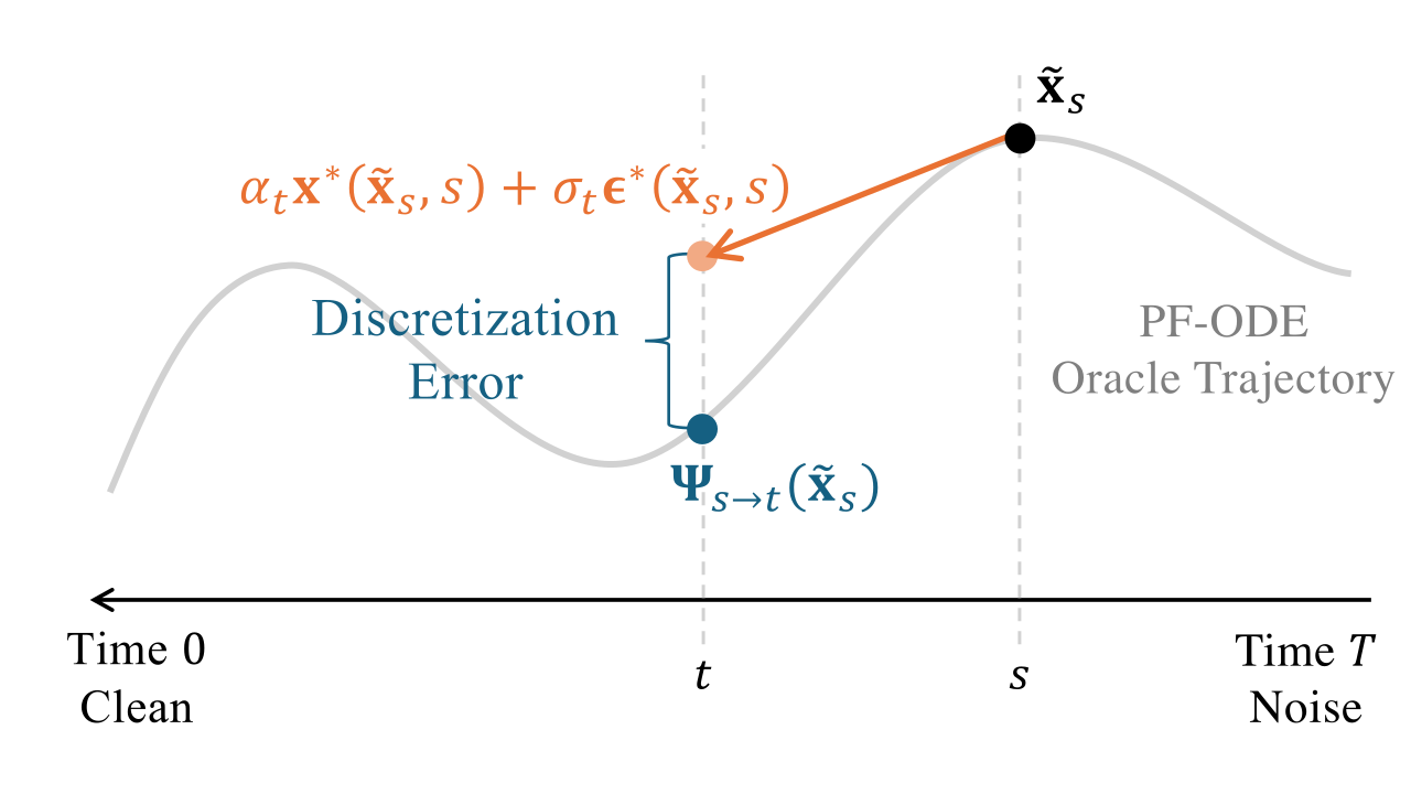
Why Does the Prediction Held Fixed Matter?
At any fixed state and time, the standard prediction parameterizations are algebraically equivalent through Equation in Chapter 6. A finite-step solver, however, introduces an additional approximation by holding one chosen prediction fixed over an interval. Such a freezing approximation is preserved under a change of parameterization only when the converted prediction also remains constant along the resulting approximate trajectory.
DDIM provides a particularly clean example. Let \[\widehat{\mathbf{x}}_0 := {\mathbf{x}}_{\bm{\phi}^\times}(\tilde{\mathbf{x}}_s,s), \qquad \widehat{\bm{\epsilon}} := {\bm{\epsilon}}_{\bm{\phi}^\times}(\tilde{\mathbf{x}}_s,s),\] where, if only one quantity is directly predicted by the model, the other is defined by the algebraic conversion in Equation in Chapter 6. Hence, by construction, \(\tilde{\mathbf{x}}_s=\alpha_s\widehat{\mathbf{x}}_0+\sigma_s\widehat{\bm{\epsilon}}\).
Holding this start-time clean/noise pair fixed defines the DDIM interpolation over the entire step: \[\tilde{\mathbf{x}}_\tau^{\mathrm{DDIM}} = \alpha_\tau\widehat{\mathbf{x}}_0 + \sigma_\tau\widehat{\bm{\epsilon}}, \qquad \tau\in[t,s].\] This requires no additional model evaluations: once \((\widehat{\mathbf{x}}_0,\widehat{\bm{\epsilon}})\) is fixed at time \(s\), the schedule coefficients \((\alpha_\tau,\sigma_\tau)\) are known for every intermediate \(\tau\). At \(\tau=s\) the expression recovers the starting state, while at \(\tau=t\) it gives the DDIM update. The intermediate values simply describe the finite-step trajectory induced by the DDIM approximation.
The special role of noise and clean-data prediction is now immediate. Along this trajectory, \[\frac{ \tilde{\mathbf{x}}_\tau^{\mathrm{DDIM}} - \sigma_\tau\widehat{\bm{\epsilon}} }{ \alpha_\tau } = \widehat{\mathbf{x}}_0, \qquad \frac{ \tilde{\mathbf{x}}_\tau^{\mathrm{DDIM}} - \alpha_\tau\widehat{\mathbf{x}}_0 }{ \sigma_\tau } = \widehat{\bm{\epsilon}}.\] Thus, the algebraically converted clean and noise predictions remain constant together along the DDIM trajectory. Consequently, holding \({\bm{\epsilon}}_{\bm{\phi}^\times}({\mathbf{x}}_\tau,\tau) \approx{\bm{\epsilon}}_{\bm{\phi}^\times}(\tilde{\mathbf{x}}_s,s)\) or holding \({\mathbf{x}}_{\bm{\phi}^\times}({\mathbf{x}}_\tau,\tau) \approx{\mathbf{x}}_{\bm{\phi}^\times}(\tilde{\mathbf{x}}_s,s)\) leads to the same DDIM update. In this sense, \(\widehat{\mathbf{x}}_0\) and \(\widehat{\bm{\epsilon}}\) are the two fixed components of the DDIM shared-noise path, while \((\alpha_\tau,\sigma_\tau)\) provide the known time-dependent weights.
However, score and velocity behave differently. DDIM keeps the inferred clean/noise pair \((\widehat{\mathbf{x}}_0,\widehat{\bm{\epsilon}})\) fixed, but the score and velocity obtained from this pair generally change with time.
For example, converting the fixed (at time \(s\)) noise estimate to score prediction at an intermediate time \(\tau\) gives \[{\mathbf{s}}(\tilde{\mathbf{x}}_\tau^{\mathrm{DDIM}},\tau) = -\frac{\widehat{\bm{\epsilon}}}{\sigma_\tau} = \frac{\sigma_s}{\sigma_\tau} {\mathbf{s}}_{\bm{\phi}^\times}(\tilde{\mathbf{x}}_s,s).\] Thus, even though \(\widehat{\bm{\epsilon}}\) is fixed, its corresponding score generally varies with \(\tau\) through the factor \(1/\sigma_\tau\). Directly imposing \[{\mathbf{s}}_{\bm{\phi}^\times}({\mathbf{x}}_\tau,\tau) \approx {\mathbf{s}}_{\bm{\phi}^\times}(\tilde{\mathbf{x}}_s,s), \qquad \tau\in[t,s],\] therefore makes a different finite-step approximation and generally yields a different first-order factored solver. Similarly, the fixed clean/noise pair induces the velocity \[\frac{\mathop{}\!\mathrm{d}}{\mathop{}\!\mathrm{d}\tau} \tilde{\mathbf{x}}_\tau^{\mathrm{DDIM}} = \alpha_\tau'\widehat{\mathbf{x}}_0 + \sigma_\tau'\widehat{\bm{\epsilon}}.\] This velocity generally changes with \(\tau\) because the schedule derivatives \(\alpha_\tau'\) and \(\sigma_\tau'\) change. Holding the raw velocity prediction fixed instead, \({\mathbf{v}}_{\bm{\phi}^\times}({\mathbf{x}}_\tau,\tau) \approx {\mathbf{v}}_{\bm{\phi}^\times}(\tilde{\mathbf{x}}_s,s)\), gives plain Euler in the original diffusion time; its relation to DDIM is discussed in Section 1.2.2.
Remark. Prediction parameterizations are pointwise algebraically equivalent, but finite-step freezing need not commute with a time-dependent conversion. DDIM keeps a consistent start-time clean/noise pair fixed; the corresponding score and complete velocity generally vary over the step. Hence directly freezing the raw score or velocity defines a different first-order method. The velocity case is quantified in Section 1.2.2.
Relation to Euler-Type Methods
The discussion above shows that DDIM is a first-order method, but its relation to the classical Euler method requires some care. Once the known diffusion schedule is separated from the learned prediction, different first-order schemes arise depending on what is held fixed over a finite step.
We compare three one-evaluation constructions:
plain Euler, which holds the complete PF-ODE velocity fixed;
exponential Euler, which treats the known linear propagation analytically but holds the remaining coefficient-weighted residual fixed;
DDIM, which keeps the start-time clean/noise estimates fixed while retaining their finite-step evolution under the known diffusion schedule.
These distinctions are easiest to see from two equivalent views of the same DDIM update. The clean/noise form makes its difference from plain Euler transparent, whereas the factored semilinear form clarifies its relation to exponential Euler. We then identify the remaining discretization error and show the precise sense in which DDIM itself can be viewed as an Euler method after a schedule-aligned change of coordinates.
DDIM versus Plain Euler.
DDIM and plain Euler use the same start-time model information, but propagate it differently over a finite step. Plain Euler locally approximates the complete PF-ODE velocity, whereas DDIM retains the finite-step evolution of the known diffusion schedule while holding the model prediction fixed. Consequently, for smooth schedules, the two updates agree to first order and generally differ by terms of order \(\mathcal O((\Delta s)^2)\). We make this difference explicit below.
Consider one backward step from time \(s\) to \(t<s\), with \(\Delta s:=s-t>0\), and suppose the start-time clean and noise predictions are algebraically consistent: \[\tilde{\mathbf{x}}_s = \alpha_s {\mathbf{x}}_{\bm{\phi}^\times}(\tilde{\mathbf{x}}_s,s) + \sigma_s {\bm{\epsilon}}_{\bm{\phi}^\times}(\tilde{\mathbf{x}}_s,s).\] The corresponding empirical PF-ODE velocity at time \(s\) is \[{\mathbf{v}}_{\bm{\phi}^\times}(\tilde{\mathbf{x}}_s,s) = \alpha_s' {\mathbf{x}}_{\bm{\phi}^\times}(\tilde{\mathbf{x}}_s,s) + \sigma_s' {\bm{\epsilon}}_{\bm{\phi}^\times}(\tilde{\mathbf{x}}_s,s).\] Plain Euler holds this complete velocity fixed over the step, \(\tau\in[t,s]\), and gives: \[\tilde{\mathbf{x}}_t^{\mathrm{Euler}} = \tilde{\mathbf{x}}_s - \Delta s\, {\mathbf{v}}_{\bm{\phi}^\times}(\tilde{\mathbf{x}}_s,s).\] By contrast, DDIM keeps the clean/noise-prediction pair at the starting time fixed, while evolving the known schedule coefficients from \((\alpha_s,\sigma_s)\) to \((\alpha_t,\sigma_t)\): \[\tilde{\mathbf{x}}_t^{\mathrm{DDIM}} = \tilde{\mathbf{x}}_s + (\alpha_t-\alpha_s) {\mathbf{x}}_{\bm{\phi}^\times}(\tilde{\mathbf{x}}_s,s) + (\sigma_t-\sigma_s) {\bm{\epsilon}}_{\bm{\phi}^\times}(\tilde{\mathbf{x}}_s,s).\] Their exact finite-step difference is therefore \[\begin{align*} \tilde{\mathbf{x}}_t^{\mathrm{DDIM}} - \tilde{\mathbf{x}}_t^{\mathrm{Euler}} ={}& \left[ \alpha_t-\alpha_s+\Delta s\,\alpha_s' \right] {\mathbf{x}}_{\bm{\phi}^\times}(\tilde{\mathbf{x}}_s,s) + \left[ \sigma_t-\sigma_s+\Delta s\,\sigma_s' \right] {\bm{\epsilon}}_{\bm{\phi}^\times}(\tilde{\mathbf{x}}_s,s). \end{align*}\] For smooth schedules, \[\alpha_t-\alpha_s+\Delta s\,\alpha_s' = \tfrac{(\Delta s)^2}{2}\alpha_s'' + \mathcal O((\Delta s)^3), \quad \sigma_t-\sigma_s+\Delta s\,\sigma_s' = \tfrac{(\Delta s)^2}{2}\sigma_s'' + \mathcal O((\Delta s)^3).\] Hence, \[\begin{align*} \tilde{\mathbf{x}}_t^{\mathrm{DDIM}} - \tilde{\mathbf{x}}_t^{\mathrm{Euler}} = \tfrac{(\Delta s)^2}{2} \left[ \alpha_s'' {\mathbf{x}}_{\bm{\phi}^\times}(\tilde{\mathbf{x}}_s,s) + \sigma_s'' {\bm{\epsilon}}_{\bm{\phi}^\times}(\tilde{\mathbf{x}}_s,s) \right] + \mathcal O((\Delta s)^3). \end{align*}\] Thus, DDIM and plain Euler agree to first order but generally differ over a finite step. Plain Euler replaces the finite schedule changes \((\alpha_t-\alpha_s,\sigma_t-\sigma_s)\) by their local linearizations, whereas DDIM retains the finite schedule evolution analytically.
A useful special case follows immediately. If both \(\alpha_\tau\) and \(\sigma_\tau\) are affine in \(\tau\) over \([t,s]\), then \[\alpha_t-\alpha_s=-\Delta s\,\alpha_s', \qquad \sigma_t-\sigma_s=-\Delta s\,\sigma_s',\] so DDIM and plain Euler coincide exactly. This includes, for example, the schedules (see also discussion in Section ((Optional) Analysis of Parametrizations and the Canonical Flow) in Chapter 6) \[(\alpha_t,\sigma_t)=(1,t)\quad \text{and}\quad (\alpha_t,\sigma_t)=(1-t,t) .\] Thus, the finite-step distinction between the two methods is driven by the nonlinearity of the known schedule in the original diffusion time.
DDIM versus Exponential Euler.
The comparison above used the clean/noise representation to show how DDIM differs from plain Euler in the original diffusion time. We now return to the semilinear representation from the prologue to distinguish DDIM from conventional exponential Euler. The difference is simple: both methods retain the known linear evolution analytically, but they hold different quantities fixed inside the remaining integral.
Under noise prediction, the factored PF-ODE in Equation \(\eqref{eq:general-semilinear-pfode}\) has \[a(\tau)=f(\tau), \qquad b(\tau)=\frac{g^2(\tau)}{2\sigma_\tau}, \qquad {\mathbf{N}}_{\bm{\phi}^\times} = {\bm{\epsilon}}_{\bm{\phi}^\times}.\] Its exact variation-of-constants formula contains the model-dependent term \[b(\tau){\bm{\epsilon}}_{\bm{\phi}^\times}({\mathbf{x}}_\tau,\tau).\]
Conventional exponential Euler treats this coefficient-weighted quantity as a single residual and holds the whole residual fixed at the beginning of the step: \[b(\tau){\bm{\epsilon}}_{\bm{\phi}^\times}({\mathbf{x}}_\tau,\tau) \approx b(s){\bm{\epsilon}}_{\bm{\phi}^\times}(\tilde{\mathbf{x}}_s,s), \quad\tau\in[t,s]\] It therefore gives \[\tilde{\mathbf{x}}_t^{\mathrm{ExpEuler}} = \mathcal E(s\rightarrow t)\tilde{\mathbf{x}}_s + b(s) \left[ \int_s^t \mathcal E(\tau\rightarrow t) \mathop{}\!\mathrm{d}\tau \right] {\bm{\epsilon}}_{\bm{\phi}^\times}(\tilde{\mathbf{x}}_s,s).\]
DDIM uses the finer factorization emphasized in the prologue. Since \(b(\tau)\) is known from the diffusion schedule, it remains inside the integral; only the neural prediction is held fixed: \[{\bm{\epsilon}}_{\bm{\phi}^\times}({\mathbf{x}}_\tau,\tau) \approx {\bm{\epsilon}}_{\bm{\phi}^\times}(\tilde{\mathbf{x}}_s,s).\] Hence, \[\tilde{\mathbf{x}}_t^{\mathrm{DDIM}} = \mathcal E(s\rightarrow t)\tilde{\mathbf{x}}_s + \left[ \int_s^t \mathcal E(\tau\rightarrow t)b(\tau) \mathop{}\!\mathrm{d}\tau \right] {\bm{\epsilon}}_{\bm{\phi}^\times}(\tilde{\mathbf{x}}_s,s).\]
The finite-step difference between the two updates therefore comes entirely from the known coefficient \(b(\tau)\): \[\tilde{\mathbf{x}}_t^{\mathrm{DDIM}} - \tilde{\mathbf{x}}_t^{\mathrm{ExpEuler}} = \left[ \int_s^t \mathcal E(\tau\rightarrow t) \bigl(b(\tau)-b(s)\bigr) \mathop{}\!\mathrm{d}\tau \right] {\bm{\epsilon}}_{\bm{\phi}^\times}(\tilde{\mathbf{x}}_s,s).\] For smooth \(b\), \[\tilde{\mathbf{x}}_t^{\mathrm{DDIM}} - \tilde{\mathbf{x}}_t^{\mathrm{ExpEuler}} = \frac{(\Delta s)^2}{2} b'(s) {\bm{\epsilon}}_{\bm{\phi}^\times}(\tilde{\mathbf{x}}_s,s) + \mathcal O((\Delta s)^3).\] Thus, DDIM and conventional exponential Euler agree to first order. The only difference is that exponential Euler freezes \(b(\tau)\) at \(b(s)\) together with the neural prediction, while DDIM keeps the known variation of \(b(\tau)\). Therefore, the two updates coincide exactly whenever \(b(\tau)\) is constant over the step, including the constant-\(b\) setting used in the Prologue example.
Together with the preceding plain-Euler comparison, the three first-order rules differ only in how much known structure is retained before making the constant approximation on \(\tau\in[t,s]\): \[\begin{array}{rcl} \text{Plain Euler} &:& f(\tau){\mathbf{x}}_\tau+b(\tau){\bm{\epsilon}}_\tau \;\approx\; f(s)\tilde{\mathbf{x}}_s+b(s)\widehat{\bm{\epsilon}}, \\[4pt] \text{Exponential Euler} &:& b(\tau){\bm{\epsilon}}_\tau \;\approx\; b(s)\widehat{\bm{\epsilon}}, \\[4pt] \text{DDIM} &:& {\bm{\epsilon}}_\tau \;\approx\; \widehat{\bm{\epsilon}}, \end{array}\] where \(\widehat{\bm{\epsilon}} := {\bm{\epsilon}}_{\bm{\phi}^\times}(\tilde{\mathbf{x}}_s,s)\). All three use the same single neural-network evaluation at the beginning of the step. Plain Euler approximates the complete velocity; exponential Euler first retains the known linear propagation; DDIM additionally retains the known coefficient \(b(\tau)\) and approximates only the neural prediction.
This hierarchy concerns which analytically known terms are preserved, rather than a universal ordering of one-step errors. Its main numerical consequence is that the remaining approximation in DDIM can be isolated entirely to the variation of the neural prediction, as we show next.
What Error Does Each Method Still Make?
The comparisons above describe how the three numerical updates differ from one another. We now compare each update with the exact empirical PF-ODE flow. For this local-error analysis, suppose the step starts from an exact empirical state \({\mathbf{x}}_s\) at time \(s\).
For plain Euler, the exact empirical flow can be written in the direct velocity form as \[\widetilde{\bm{\Psi}}_{s\to t}({\mathbf{x}}_s) = {\mathbf{x}}_s + \int_s^t {\mathbf{v}}_{\bm{\phi}^\times}({\mathbf{x}}_\tau,\tau) \mathop{}\!\mathrm{d}\tau.\] Since plain Euler holds the complete velocity fixed at its start-time value, its exact one-step defect is \[\begin{align*} \widetilde{\bm{\Psi}}_{s\to t}({\mathbf{x}}_s) - \tilde{\mathbf{x}}_t^{\mathrm{Euler}} = \int_s^t \Big[ {\mathbf{v}}_{\bm{\phi}^\times}({\mathbf{x}}_\tau,\tau) - {\mathbf{v}}_{\bm{\phi}^\times}({\mathbf{x}}_s,s) \Big] \mathop{}\!\mathrm{d}\tau. \end{align*}\]
For exponential Euler, the known linear propagation is already treated analytically, but the coefficient-weighted residual \(b(\tau){\bm{\epsilon}}_{\bm{\phi}^\times}({\mathbf{x}}_\tau,\tau)\) is held fixed. Hence \[\begin{align*} \widetilde{\bm{\Psi}}_{s\to t}({\mathbf{x}}_s) - \tilde{\mathbf{x}}_t^{\mathrm{ExpEuler}} = \int_s^t \mathcal E(\tau\rightarrow t) \Big[ b(\tau) {\bm{\epsilon}}_{\bm{\phi}^\times}({\mathbf{x}}_\tau,\tau) - b(s) {\bm{\epsilon}}_{\bm{\phi}^\times}({\mathbf{x}}_s,s) \Big] \mathop{}\!\mathrm{d}\tau. \end{align*}\]
Finally, DDIM retains both the known linear propagation and the known coefficient \(b(\tau)\), and holds only the neural prediction fixed: \[\begin{align} \label{eq:ddim-local-defect} \widetilde{\bm{\Psi}}_{s\to t}({\mathbf{x}}_s) - \tilde{\mathbf{x}}_t^{\mathrm{DDIM}} = \int_s^t \mathcal E(\tau\rightarrow t)b(\tau) \Big[ {\bm{\epsilon}}_{\bm{\phi}^\times}({\mathbf{x}}_\tau,\tau) - {\bm{\epsilon}}_{\bm{\phi}^\times}({\mathbf{x}}_s,s) \Big] \mathop{}\!\mathrm{d}\tau. \end{align}\]
These identities reveal the relevant notion of smoothness for each first-order scheme. If the corresponding quantity varies slowly along the exact empirical trajectory, then the one-step approximation is accurate. More precisely, with \(\Delta s:=s-t\), standard smoothness gives \[\begin{align*} \left\| \widetilde{\bm{\Psi}}_{s\to t}({\mathbf{x}}_s) - \tilde{\mathbf{x}}_t^{\mathrm{Euler}} \right\| &\le \frac{(\Delta s)^2}{2} \sup_{\tau\in[t,s]} \left\| \tfrac{\mathop{}\!\mathrm{d}}{\mathop{}\!\mathrm{d}\tau} {\mathbf{v}}_{\bm{\phi}^\times}({\mathbf{x}}_\tau,\tau) \right\|, \\ \left\| \widetilde{\bm{\Psi}}_{s\to t}({\mathbf{x}}_s) - \tilde{\mathbf{x}}_t^{\mathrm{ExpEuler}} \right\| &\le \frac{(\Delta s)^2}{2} \sup_{\tau\in[t,s]} \left| \mathcal E(\tau\rightarrow t) \right|\cdot \sup_{\tau\in[t,s]} \left\| \tfrac{\mathop{}\!\mathrm{d}}{\mathop{}\!\mathrm{d}\tau} \left[ b(\tau) {\bm{\epsilon}}_{\bm{\phi}^\times}({\mathbf{x}}_\tau,\tau) \right] \right\|, \\ \left\| \widetilde{\bm{\Psi}}_{s\to t}({\mathbf{x}}_s) - \tilde{\mathbf{x}}_t^{\mathrm{DDIM}} \right\| &\le \frac{(\Delta s)^2}{2} \sup_{\tau\in[t,s]} \left| \mathcal E(\tau\rightarrow t)b(\tau) \right| \cdot \sup_{\tau\in[t,s]} \left\| \tfrac{\mathop{}\!\mathrm{d}}{\mathop{}\!\mathrm{d}\tau} {\bm{\epsilon}}_{\bm{\phi}^\times}({\mathbf{x}}_\tau,\tau) \right\|. \end{align*}\]
Under the usual smoothness and stability assumptions, all three methods are globally first order and require only one neural-network evaluation per step. Moreover, each method is exact on a step when the quantity it holds fixed is in fact constant along the exact empirical trajectory: the complete PF-ODE velocity for plain Euler, the coefficient-weighted residual \(b(\tau){\bm{\epsilon}}_{\bm{\phi}^\times}({\mathbf{x}}_\tau,\tau)\) for exponential Euler, and the noise prediction \({\bm{\epsilon}}_{\bm{\phi}^\times}({\mathbf{x}}_\tau,\tau)\) for DDIM.
Accordingly, there is no universal error ordering among the three methods: each is most accurate when the quantity it holds fixed varies slowly over the step. DDIM is particularly well suited to regimes where the neural prediction changes slowly but the known diffusion schedule changes appreciably, since it retains the latter analytically. Exploiting more known structure can therefore reduce discretization error, but does not guarantee a smaller error on every individual step.
The errors discussed here are numerical discretization errors relative to the empirical PF-ODE; model mismatch between the empirical and oracle PF-ODEs is a separate source of error.
A Precise Euler Interpretation of DDIM.
Although DDIM and plain Euler agree to first order, they generally give different finite-step updates in the original state \({\mathbf{x}}\) and diffusion time \(t\). There is, however, an exact Euler interpretation after a schedule-aligned change of both the state and the time coordinate.
Under noise prediction, define \[\begin{equation*} {\mathbf{y}}_t := \frac{{\mathbf{x}}_t}{\alpha_t}, \qquad \rho_t := \frac{\sigma_t}{\alpha_t}. \end{equation*}\] The two transformations play complementary roles. The state normalization \({\mathbf{x}}_t\mapsto{\mathbf{x}}_t/\alpha_t\) factors out the known signal scaling \(\alpha_t\), while the new clock \(\rho_t=\sigma_t/\alpha_t\) measures progress by the noise-to-signal ratio rather than by the original diffusion time.
To see this first at the conditional level, consider a fixed pair \(({\mathbf{x}}_0,{\bm{\epsilon}})\) in the Gaussian perturbation path \[{\mathbf{x}}_t = \alpha_t{\mathbf{x}}_0+\sigma_t{\bm{\epsilon}}, \qquad {\bm{\epsilon}}\sim\mathcal N(\mathbf 0,\mathbf I).\] Here, \({\bm{\epsilon}}\) is a fixed latent noise realization, not a neural prediction. The transformed state satisfies \[{\mathbf{y}}_t = \frac{{\mathbf{x}}_t}{\alpha_t} = {\mathbf{x}}_0+\rho_t{\bm{\epsilon}}.\] Hence, along this particular conditional path, \[\frac{\mathop{}\!\mathrm{d}{\mathbf{y}}}{\mathop{}\!\mathrm{d}\rho} = {\bm{\epsilon}}.\] Thus, for fixed \(({\mathbf{x}}_0,{\bm{\epsilon}})\), the known schedule dependence becomes affine in the transformed coordinate \(\rho\).
The corresponding empirical PF-ODE has the same coordinate structure, but the fixed latent noise \({\bm{\epsilon}}\) is replaced by the learned, state-dependent noise prediction. Using Equation \(\eqref{eq:noise_pf_ode}\), \[\frac{\mathop{}\!\mathrm{d}{\mathbf{x}}_t}{\mathop{}\!\mathrm{d}t} = \frac{\alpha_t'}{\alpha_t}{\mathbf{x}}_t + \left( \sigma_t' - \frac{\alpha_t'}{\alpha_t}\sigma_t \right) {\bm{\epsilon}}_{\bm{\phi}^\times}({\mathbf{x}}_t,t),\] we obtain \[\begin{align} \frac{\mathop{}\!\mathrm{d}{\mathbf{y}}_t}{\mathop{}\!\mathrm{d}t} = \frac{1}{\alpha_t} \left( \frac{\mathop{}\!\mathrm{d}{\mathbf{x}}_t}{\mathop{}\!\mathrm{d}t} - \frac{\alpha_t'}{\alpha_t}{\mathbf{x}}_t \right)= \frac{\mathop{}\!\mathrm{d}\rho_t}{\mathop{}\!\mathrm{d}t}\, {\bm{\epsilon}}_{\bm{\phi}^\times}({\mathbf{x}}_t,t). \label{eq:ddim-coordinate-ode-t} \end{align}\] Hence, on any interval where \(\alpha_t>0\) and \(\rho_t\) is strictly monotone, we may use \(\rho\) as the time coordinate. Writing \(t=t(\rho)\) and defining the transformed neural field \[\bar{{\bm{\epsilon}}}_{\bm{\phi}^\times}({\mathbf{y}},\rho) := {\bm{\epsilon}}_{\bm{\phi}^\times} \bigl( \alpha_{t(\rho)}{\mathbf{y}}, t(\rho) \bigr),\] the empirical PF-ODE becomes \[\begin{equation} \label{eq:ddim-coordinate-ode-rho} \frac{\mathop{}\!\mathrm{d}{\mathbf{y}}}{\mathop{}\!\mathrm{d}\rho} = \bar{{\bm{\epsilon}}}_{\bm{\phi}^\times}({\mathbf{y}},\rho). \end{equation}\] The spatial and temporal dependence of the model therefore remains present; it is simply expressed in the transformed variables \(({\mathbf{y}},\rho)\).
Explicit Euler applied to Equation \(\eqref{eq:ddim-coordinate-ode-rho}\) from \(\rho_s\) to \(\rho_t\) gives \[\tilde{\mathbf{y}}_t = \tilde{\mathbf{y}}_s + (\rho_t-\rho_s) \bar{{\bm{\epsilon}}}_{\bm{\phi}^\times}(\tilde{\mathbf{y}}_s,\rho_s).\] Since \[\bar{{\bm{\epsilon}}}_{\bm{\phi}^\times}(\tilde{\mathbf{y}}_s,\rho_s) = {\bm{\epsilon}}_{\bm{\phi}^\times}(\tilde{\mathbf{x}}_s,s),\] substituting \({\mathbf{y}}={\mathbf{x}}/\alpha\) and \(\rho=\sigma/\alpha\) yields \[\tilde{\mathbf{x}}_t = \frac{\alpha_t}{\alpha_s}\tilde{\mathbf{x}}_s + \alpha_t \left( \frac{\sigma_t}{\alpha_t} - \frac{\sigma_s}{\alpha_s} \right) {\bm{\epsilon}}_{\bm{\phi}^\times}(\tilde{\mathbf{x}}_s,s),\] which is exactly the deterministic DDIM update.
Coordinate Choice Is Part of the Numerical Method
An invertible change of state and time coordinates gives an equivalent representation of the same continuous ODE solution. A finite-step discretization, however, is generally not invariant to that representation: “change coordinates and then apply Euler” need not equal “apply Euler and then change coordinates”.
The numerical significance is that a suitable coordinate system can absorb analytically known parts of the dynamics before discretization. In DDIM, \({\mathbf{x}}/\alpha\) removes the known signal scaling and \(\rho=\sigma/\alpha\) absorbs the corresponding schedule-dependent time scaling, leaving the transformed neural field \(\bar{{\bm{\epsilon}}}_{\bm{\phi}^\times}({\mathbf{y}},\rho)\) as the quantity approximated by Euler. Thus DDIM generally differs from plain Euler in \(({\mathbf{x}},t)\), while it is exactly explicit Euler in the schedule-aligned coordinates \(({\mathbf{y}},\rho)\).
A dual construction holds under clean-data prediction. Normalizing the state by \(\sigma_t\) and using \(\alpha_t/\sigma_t\) as the time coordinate gives \[\frac{\mathop{}\!\mathrm{d}}{\mathop{}\!\mathrm{d}t} \left( \frac{{\mathbf{x}}_t}{\sigma_t} \right) = \frac{\mathop{}\!\mathrm{d}}{\mathop{}\!\mathrm{d}t} \left( \frac{\alpha_t}{\sigma_t} \right) {\mathbf{x}}_{\bm{\phi}^\times}({\mathbf{x}}_t,t),\] so the clean-data form of DDIM is likewise explicit Euler in its corresponding schedule-aligned coordinates.
This state–time change-of-coordinates viewpoint also previews the role of coordinate choice in higher-order diffusion solvers. DPM-Solver, developed later in Section 1.4, uses the half-log SNR \[\lambda_t := \log\frac{\alpha_t}{\sigma_t},\] which is directly related to DDIM’s Euler clock: \[\rho_t = \frac{\sigma_t}{\alpha_t} = e^{-\lambda_t}, \qquad \mathop{}\!\mathrm{d}\rho = -e^{-\lambda}\mathop{}\!\mathrm{d}\lambda.\] Therefore, the exact transformed equation \[\frac{\mathop{}\!\mathrm{d}{\mathbf{y}}}{\mathop{}\!\mathrm{d}\rho} = \bar{{\bm{\epsilon}}}_{\bm{\phi}^\times}({\mathbf{y}},\rho)\] can equivalently be integrated as \[{\mathbf{y}}_t = {\mathbf{y}}_s - \int_{\lambda_s}^{\lambda_t} e^{-\lambda} \hat{{\bm{\epsilon}}}_{\bm{\phi}^\times} (\hat{\mathbf{x}}_\lambda,\lambda) \mathop{}\!\mathrm{d}\lambda,\] with the usual \(\lambda\)-parameterized model notation introduced later in Section 1.4.
At first order, holding the neural prediction fixed while retaining the known change-of-variable weight gives the same finite-step update, so DPM-Solver-1 is exactly DDIM. Beyond first order, however, the coordinate in which the state–time-dependent neural prediction is approximated becomes part of the numerical method. DPM-Solver uses \(\lambda\) because it yields an exponentially weighted integral with convenient higher-order expansions.
(Optional) The Original Variational Perspective on DDIM
The PF-ODE perspective above explains deterministic DDIM as a numerical solver. Historically, however, DDIM was introduced from the variational viewpoint of DDPM. Its starting question is different: does the denoising objective uniquely determine how noisy states at different times must be coupled?
Revisiting DDPM’s Variational View.
Recall that DDPM introduces a fixed Markovian inference process whose one-time perturbation marginals take the Gaussian form \[p_t({\mathbf{x}}_t|{\mathbf{x}}_0) = \mathcal N \bigl( {\mathbf{x}}_t; \alpha_t{\mathbf{x}}_0, \sigma_t^2{\mathbf{I}} \bigr).\] The corresponding variational derivation involves tractable conditionals such as \(p({\mathbf{x}}_t|{\mathbf{x}}_s,{\mathbf{x}}_0)\) for \(t<s\), while the learned reverse model used for generation cannot condition directly on the unknown clean sample \({\mathbf{x}}_0\) and instead relies on the diffusion-model prediction.
The key observation behind DDIM concerns the denoising objective. We recall that a noise-prediction DDPM loss can be written as \[\mathbb{E}_t \mathbb{E}_{{\mathbf{x}}_0,{\bm{\epsilon}}} \left[ \left\| {\bm{\epsilon}}_{\bm{\phi}} \bigl( \alpha_t{\mathbf{x}}_0+\sigma_t{\bm{\epsilon}},t \bigr) - {\bm{\epsilon}} \right\|_2^2 \right],\] which depends on the inference process through the one-time marginals \(p_t({\mathbf{x}}_t|{\mathbf{x}}_0)\), rather than through the full joint coupling of \({\mathbf{x}}_1,\ldots,{\mathbf{x}}_T\) conditioned on \({\mathbf{x}}_0\).
Original DDIM Motivation.
The central observation behind DDIM is that the denoising training objective does not uniquely determine how noisy states at different times are coupled. For a fixed clean sample \({\mathbf{x}}_0\), the usual denoising surrogate is determined by the one-time perturbation marginals \(p_t({\mathbf{x}}_t|{\mathbf{x}}_0)\), whereas many different joint processes across time can share exactly the same marginals. DDIM exploits this freedom: it preserves the perturbation marginals used during training, while changing the coupling between different noise levels.
Concretely, for any \(t<s\), consider a conditional transition \({\color{orange}\pi({\mathbf{x}}_t|{\mathbf{x}}_s,{\mathbf{x}}_0)}\). We require it to be one-step marginally consistent:
\[\begin{align} \label{eq:ddim-reverse-kernel-def} \int {\color{orange}\pi({\mathbf{x}}_t|{\mathbf{x}}_s,{\mathbf{x}}_0)} \,p_s({\mathbf{x}}_s|{\mathbf{x}}_0) \mathop{}\!\mathrm{d}{\mathbf{x}}_s = p_t({\mathbf{x}}_t|{\mathbf{x}}_0). \end{align}\]
In words, if \({\mathbf{x}}_s\sim p_s(\cdot|{\mathbf{x}}_0)\), then applying the chosen transition once produces \({\mathbf{x}}_t\sim p_t(\cdot|{\mathbf{x}}_0)\). Hence, the marginal distribution at each noise level is preserved even though the dependence between \({\mathbf{x}}_s\) and \({\mathbf{x}}_t\) may be changed.
The Bayesian reverse posterior induced by the original Markovian DDPM forward process is one valid choice of such a transition,6 but it is not uniquely determined by the marginals. DDIM instead allows other marginal-consistent couplings, including transitions directly between widely separated noise levels. This is the probabilistic reason that the same trained denoiser can be reused on a coarser sampling grid with skipped intermediate times.
Derivation of Discrete-Time DDIM.
We now make the coupling freedom above explicit for the Gaussian perturbation model \[p_t({\mathbf{x}}_t|{\mathbf{x}}_0) := \mathcal{N} \bigl( {\mathbf{x}}_t; \alpha_t{\mathbf{x}}_0, \sigma_t^2\mathbf{I} \bigr), \qquad {\mathbf{x}}_0\sim p_{\mathrm{data}}.\] The goal is to construct, for any \(t<s\), a conditional transition \({\color{orange}\pi({\mathbf{x}}_t|{\mathbf{x}}_s,{\mathbf{x}}_0)}\) that satisfies the marginal-consistency condition in Equation \(\eqref{eq:ddim-reverse-kernel-def}\), without requiring it to coincide with the Bayesian posterior associated with the original Markov forward process.
A natural choice is the Gaussian family \[\begin{align} \label{eq:ddim-reverse-kernel-param} {\color{orange}\pi({\mathbf{x}}_t|{\mathbf{x}}_s,{\mathbf{x}}_0)} = \mathcal{N} \bigl( {\mathbf{x}}_t;\, a_{t,s}{\mathbf{x}}_0+b_{t,s}{\mathbf{x}}_s,\, c_{t,s}^2\mathbf{I} \bigr), \end{align}\] where \((a_{t,s},b_{t,s},c_{t,s})\) determine how the state at time \(s\), the clean sample, and newly injected noise are combined.
To impose marginal consistency, first draw \[{\mathbf{x}}_s = \alpha_s{\mathbf{x}}_0+\sigma_s{\bm{\epsilon}}', \qquad {\bm{\epsilon}}'\sim\mathcal{N}(\mathbf{0},\mathbf{I}),\] and then draw \({\mathbf{x}}_t\) from Equation \(\eqref{eq:ddim-reverse-kernel-param}\). Equivalently, \[\begin{align} \label{eq:ddim-derivation} \begin{aligned} {\mathbf{x}}_t &= a_{t,s}{\mathbf{x}}_0 + b_{t,s}{\mathbf{x}}_s + c_{t,s}{\bm{\epsilon}} \\ &= a_{t,s}{\mathbf{x}}_0 + b_{t,s} \bigl( \alpha_s{\mathbf{x}}_0+\sigma_s{\bm{\epsilon}}' \bigr) + c_{t,s}{\bm{\epsilon}} \\ &= \bigl( a_{t,s}+b_{t,s}\alpha_s \bigr){\mathbf{x}}_0 + \sqrt{ b_{t,s}^2\sigma_s^2+c_{t,s}^2 }\, {\bm{\epsilon}}'', \end{aligned} \end{align}\] where \({\bm{\epsilon}}\) and \({\bm{\epsilon}}'\) are independent standard Gaussian variables, and \({\bm{\epsilon}}''\) is a standard Gaussian representing their normalized linear combination.
For the resulting marginal to equal the prescribed perturbation marginal \({\mathbf{x}}_t \sim p_t({\mathbf{x}}_t|{\mathbf{x}}_0) = \mathcal{N} \bigl( {\mathbf{x}}_t; \alpha_t{\mathbf{x}}_0, \sigma_t^2\mathbf{I} \bigr)\), the means and variances must agree. Therefore, \[\begin{align*} \alpha_t &= a_{t,s}+b_{t,s}\alpha_s, \\ \sigma_t^2 &= b_{t,s}^2\sigma_s^2+c_{t,s}^2. \end{align*}\]
The important point is that these are only two constraints on the three coefficients \((a_{t,s},b_{t,s},c_{t,s})\). Hence, the prescribed marginals do not determine a unique transition between \(s\) and \(t\). We may choose \(c_{t,s}\) as a free parameter, with \(0\leq c_{t,s}\leq\sigma_t\), and solve for the remaining coefficients. Choosing the nonnegative branch gives \[\begin{align} \label{eq:ddim-coefficients} b_{t,s} &= \frac{ \sqrt{\sigma_t^2-c_{t,s}^2} }{ \sigma_s }, \qquad a_{t,s} = \alpha_t-\alpha_s b_{t,s}. \end{align}\] The nonnegative choice of \(b_{t,s}\) gives the standard DDIM coupling.
Substituting Equation \(\eqref{eq:ddim-coefficients}\) into Equation \(\eqref{eq:ddim-reverse-kernel-param}\) yields \[\begin{align} \label{eq:ddim-reverse-kernel-result} {\color{orange}\pi({\mathbf{x}}_t|{\mathbf{x}}_s,{\mathbf{x}}_0)} = \mathcal{N} \left( {\mathbf{x}}_t;\, \alpha_t{\mathbf{x}}_0 + \frac{ \sqrt{\sigma_t^2-c_{t,s}^2} }{ \sigma_s } \bigl( {\mathbf{x}}_s-\alpha_s{\mathbf{x}}_0 \bigr), \, c_{t,s}^2\mathbf{I} \right). \end{align}\]
This expression makes the coupling freedom explicit. The term \({\mathbf{x}}_s-\alpha_s{\mathbf{x}}_0\) is the noise component already present in \({\mathbf{x}}_s\), while \(c_{t,s}\) controls how much new Gaussian noise is introduced in the transition from \(s\) to \(t\). Varying \(c_{t,s}\) therefore changes the coupling between the two noise levels while preserving the same target marginal \(p_t({\mathbf{x}}_t|{\mathbf{x}}_0)\).
Remark. The chosen transition \({\color{orange}\pi({\mathbf{x}}_t|{\mathbf{x}}_s,{\mathbf{x}}_0)}\) is generally different from the Bayesian posterior associated with the original Markov forward process. That posterior is recovered by one particular choice of \(c_{t,s}\), discussed below. Other choices define different marginal-consistent couplings, including the deterministic DDIM coupling obtained when \(c_{t,s}=0\).
DDIM Sampler (Step \(s\to t\)).
The marginal-consistent kernel \({\color{orange}\pi({\mathbf{x}}_t|{\mathbf{x}}_s,{\mathbf{x}}_0)}\) in Equation \(\eqref{eq:ddim-reverse-kernel-result}\) still conditions on the unknown clean sample \({\mathbf{x}}_0\). During generation, DDIM replaces \({\mathbf{x}}_0\) by the clean-data estimate obtained from the pre-trained diffusion model. Under \({\bm{\epsilon}}\)-prediction, we define \[{\mathbf{x}}_{\bm{\phi}^\times}({\mathbf{x}}_s,s) := \frac{ {\mathbf{x}}_s - \sigma_s{\bm{\epsilon}}_{\bm{\phi}^\times}({\mathbf{x}}_s,s) }{ \alpha_s },\] and use the plug-in transition \[p_{\bm{\phi}^\times}({\mathbf{x}}_t|{\mathbf{x}}_s) := {\color{orange}\pi \bigl( {\mathbf{x}}_t \,\big|\, {\mathbf{x}}_s, {\mathbf{x}}_{\bm{\phi}^\times}({\mathbf{x}}_s,s) \bigr)}.\] Substituting this estimate into Equation \(\eqref{eq:ddim-reverse-kernel-result}\) yields
\[{\mathbf{x}}_t = \frac{\alpha_t}{\alpha_s}{\mathbf{x}}_s + \left( \sqrt{\sigma_t^2-c_{t,s}^2} - \frac{\alpha_t}{\alpha_s}\sigma_s \right) {\bm{\epsilon}}_{\bm{\phi}^\times}({\mathbf{x}}_s,s) + c_{t,s}{\bm{\epsilon}}_t, \qquad {\bm{\epsilon}}_t\sim\mathcal{N}(\mathbf{0},\mathbf{I}).\]
Thus, the model prediction determines the estimated clean/noise content carried from \(s\) to \(t\), while the free coefficient \(c_{t,s}\in[0,\sigma_t]\) controls how much new Gaussian noise is injected during the step.
To interpret this degree of freedom, it is useful to compare with the original Markov forward process. For \(t<s\), define \[\alpha_{s|t} := \frac{\alpha_s}{\alpha_t}, \qquad \sigma_{s|t}^2 := \sigma_s^2-\alpha_{s|t}^2\sigma_t^2,\] so that \[p({\mathbf{x}}_s|{\mathbf{x}}_t) = \mathcal{N} \bigl( {\mathbf{x}}_s; \alpha_{s|t}{\mathbf{x}}_t, \sigma_{s|t}^2\mathbf I \bigr).\] Gaussian conditioning gives the corresponding posterior variance \[\operatorname{Var} \bigl( {\mathbf{x}}_t|{\mathbf{x}}_s,{\mathbf{x}}_0 \bigr) = \frac{\sigma_t^2}{\sigma_s^2} \sigma_{s|t}^2\mathbf I.\] This identifies the DDPM posterior as one particular member of the marginal-consistent family above and makes the role of \(c_{t,s}\) explicit:
DDPM Step (Posterior Variance). Choosing \[c_{t,s} = \frac{\sigma_t}{\sigma_s}\sigma_{s|t}\] matches the posterior variance of the original Markov forward process. Together with the nonnegative branch in Equation \(\eqref{eq:ddim-coefficients}\), the conditional kernel \({\color{orange}\pi({\mathbf{x}}_t|{\mathbf{x}}_s,{\mathbf{x}}_0)}\) then coincides with the Bayesian posterior \(p({\mathbf{x}}_t|{\mathbf{x}}_s,{\mathbf{x}}_0)\) of that process.
Deterministic DDIM (\(\eta=0\)). At the opposite extreme, setting \(c_{t,s}=0\) removes all newly injected noise. The practical update becomes \[{\mathbf{x}}_t = \frac{\alpha_t}{\alpha_s}{\mathbf{x}}_s + \left( \sigma_t - \frac{\alpha_t}{\alpha_s}\sigma_s \right) {\bm{\epsilon}}_{\bm{\phi}^\times}({\mathbf{x}}_s,s),\] which is exactly the deterministic DDIM update derived earlier from the PF-ODE.
At the conditional level, its shared-noise interpretation is especially simple: if \({\mathbf{x}}_s=\alpha_s{\mathbf{x}}_0+\sigma_s{\bm{\epsilon}}\), then the deterministic transition gives \[{\mathbf{x}}_t = \alpha_t{\mathbf{x}}_0+\sigma_t{\bm{\epsilon}}.\] Thus, no new noise is introduced; the same pair \(({\mathbf{x}}_0,{\bm{\epsilon}})\) is carried across the step while only the known schedule coefficients change.
Interpolation. More generally, define \[\begin{align} \label{eq:eta-ddim} c_{t,s} = \eta\, \frac{\sigma_t}{\sigma_s}\, \sigma_{s|t}, \qquad \eta\in[0,1]. \end{align}\] The parameter \(\eta\) continuously controls the stochasticity of the transition: \(\eta=0\) gives deterministic DDIM, whereas \(\eta=1\) matches the posterior variance of the corresponding DDPM Markov transition.
Hence, the DDIM family separates two ingredients that are fixed differently: the perturbation marginals are kept unchanged, while the coupling between successive noise levels can be varied through \(c_{t,s}\). Deterministic DDIM corresponds to preserving the existing shared noise across the step, whereas the DDPM posterior choice injects the amount of additional randomness prescribed by the original Markov forward process.
Connection to Conditional Flow Matching.
The deterministic DDIM construction above also provides a simple connection to conditional flow matching (CFM) in Section (Flow Matching FrameworkFlow Matching Framework) in Chapter 5. The key is to distinguish two objects associated with the same conditional Gaussian path: its finite-time map and its instantaneous velocity. DDIM is related to the former, whereas CFM is built from the latter.
Condition on a clean sample \({\mathbf{x}}_0\) and consider the shared-noise path \[{\mathbf{x}}_\tau = \alpha_\tau{\mathbf{x}}_0 + \sigma_\tau{\bm{\epsilon}}.\] For fixed \(({\mathbf{x}}_0,{\bm{\epsilon}})\), this is an exact conditional trajectory through the Gaussian perturbation marginals \(p_\tau({\mathbf{x}}_\tau|{\mathbf{x}}_0)\).
Finite-Time View: the Conditional DDIM Map. Suppose the trajectory is at \({\mathbf{x}}_s\) at time \(s\). Since the same \({\bm{\epsilon}}\) is retained, eliminating it from \({\mathbf{x}}_s=\alpha_s{\mathbf{x}}_0+\sigma_s{\bm{\epsilon}}\) gives the exact conditional map \[{\bm{\Psi}}_{s\to t}({\mathbf{x}}_s|{\mathbf{x}}_0) = \frac{\sigma_t}{\sigma_s}{\mathbf{x}}_s + \left( \alpha_t - \alpha_s\frac{\sigma_t}{\sigma_s} \right){\mathbf{x}}_0.\] This map is exact conditioned on \({\mathbf{x}}_0\). It is not yet the practical DDIM sampler, because \({\mathbf{x}}_0\) is unknown during generation. Replacing \({\mathbf{x}}_0\) by its start-time model prediction gives precisely the deterministic DDIM update derived above.
Infinitesimal-Time View: the CFM Conditional Velocity. Instead of asking where the conditional path moves over a finite interval, we may ask for its instantaneous direction. Differentiating \({\mathbf{x}}_t=\alpha_t{\mathbf{x}}_0+\sigma_t{\bm{\epsilon}}\) gives \[\frac{\mathop{}\!\mathrm{d}{\mathbf{x}}_t}{\mathop{}\!\mathrm{d}t} = \alpha_t'{\mathbf{x}}_0+\sigma_t'{\bm{\epsilon}}.\] Using \[{\bm{\epsilon}} = \frac{{\mathbf{x}}-\alpha_t{\mathbf{x}}_0}{\sigma_t},\] the same velocity can be written as a function of the current state: \[{\mathbf{v}}_t^*({\mathbf{x}}|{\mathbf{x}}_0) = \frac{\sigma_t'}{\sigma_t}{\mathbf{x}} + \left( \alpha_t' - \alpha_t\frac{\sigma_t'}{\sigma_t} \right){\mathbf{x}}_0.\] This is the conditional velocity associated with the Gaussian probability path in conditional flow matching.
CFM then connects this conditional velocity to the marginal dynamics by averaging over the posterior uncertainty about \({\mathbf{x}}_0\) at the current state: \[\begin{align*} {\mathbf{v}}^*({\mathbf{x}},t) &:= \mathbb{E}_{{\mathbf{x}}_0\sim p({\mathbf{x}}_0|{\mathbf{x}}_t={\mathbf{x}})} \left[ {\mathbf{v}}_t^*({\mathbf{x}}|{\mathbf{x}}_0) \right] \\ &= \frac{\sigma_t'}{\sigma_t}{\mathbf{x}} + \left( \alpha_t' - \alpha_t\frac{\sigma_t'}{\sigma_t} \right) {\mathbf{x}}^*({\mathbf{x}},t) \\ &= \alpha_t'{\mathbf{x}}^*({\mathbf{x}},t) + \sigma_t'{\bm{\epsilon}}^*({\mathbf{x}},t), \end{align*}\] where we used \[{\mathbf{x}}^*({\mathbf{x}},t) = \mathbb{E}[{\mathbf{x}}_0|{\mathbf{x}}_t={\mathbf{x}}], \qquad {\mathbf{x}} = \alpha_t{\mathbf{x}}^*({\mathbf{x}},t) + \sigma_t{\bm{\epsilon}}^*({\mathbf{x}},t).\] The resulting \({\mathbf{v}}^*({\mathbf{x}},t)\) is exactly the oracle marginal PF-ODE velocity.
DDIM and CFM
The same conditional Gaussian path gives two views: DDIM uses its finite-time map after replacing the unknown \({\mathbf{x}}_0\) by a model prediction, while CFM uses its instantaneous conditional velocity. Posterior averaging the latter gives the marginal PF-ODE velocity.
This connection is exact at the level of the conditional path and its instantaneous velocity. It does not imply that a finite DDIM step is the exact marginal PF-ODE flow: DDIM keeps the prediction inferred at the beginning of the step fixed, whereas the exact marginal PF-ODE velocity changes continuously with the evolving state.
DEIS
In the factored exponential-integrator formula (Equation \(\eqref{eq:variation_of_constants}\)), \[\int_s^t \frac{g^2(\tau)}{2\sigma_\tau}\, \mathcal E(\tau\rightarrow t)\, {\bm{\epsilon}}_{\bm{\phi}^\times}({\mathbf{x}}_\tau,\tau) \mathop{}\!\mathrm{d}\tau,\] all schedule-dependent factors are known; the only unknown quantity along the trajectory is the neural prediction \({\bm{\epsilon}}_{\bm{\phi}^\times}({\mathbf{x}}_\tau,\tau)\). DDIM makes the simplest first-order approximation by holding this prediction fixed at the beginning of the step, \[{\bm{\epsilon}}_{\bm{\phi}^\times}({\mathbf{x}}_\tau,\tau) \approx {\bm{\epsilon}}_{\bm{\phi}^\times}({\mathbf{x}}_s,s), \qquad \tau\in[t,s].\] This approximation can become inaccurate over larger steps when the neural prediction varies appreciably along the trajectory.
DEIS (Zhang and Chen 2022) improves on this idea without introducing additional model evaluations within the current step. Inspired by classical multistep methods such as Adams–Bashforth (see Appendix A), it reuses model predictions from previous completed steps as anchors and fits a polynomial that extrapolates their recent variation into the next step. The polynomial then replaces the unknown neural prediction inside the integral, while the known schedule-dependent weight \(\tfrac{g^2(\tau)}{2\sigma_\tau} \mathcal E(\tau\rightarrow t)\) is retained analytically. Thus, DEIS extends the constant approximation of DDIM to a higher-order multistep polynomial approximation.
From the classical numerical viewpoint, DEIS is therefore an Adams–Bashforth-type multistep method within the factored exponential-integrator framework: previous neural evaluations provide the higher-order information, while the known diffusion dynamics are retained in the weighted integral.
We first review the polynomial extrapolation used to construct this approximation in Section 1.3.1, then derive the resulting DEIS update in Section 1.3.2. Finally, Section 1.3.3 shows that the constant, degree-zero case recovers DDIM.
Background: Polynomial Extrapolation
Before deriving DEIS, we briefly review the polynomial construction it uses to reuse previous model evaluations. The idea is simple: first fit a polynomial through several known values, and then evaluate that polynomial beyond the most recent anchor to predict how the quantity may continue to change. Thus, the polynomial is an interpolant at the known anchors and acts as an extrapolant over the next solver step.
From Anchors to a Polynomial Extrapolant.
Suppose a time-varying quantity is known at \(n{+}1\) distinct times, \[(\tau_0,{\mathbf{Y}}_0),\; (\tau_1,{\mathbf{Y}}_1),\; \ldots,\; (\tau_n,{\mathbf{Y}}_n), \qquad \tau_0<\tau_1<\cdots<\tau_n,\] where each \({\mathbf{Y}}_j\) may be vector-valued. We would like to construct the simplest smooth curve that exactly matches these observed values and can then be continued beyond the most recent anchor. The unique polynomial of degree at most \(n\) passing through all anchors is the Lagrange interpolant \[P_n(\tau) = \sum_{j=0}^{n} \ell_j(\tau)\,{\mathbf{Y}}_j,\] with basis functions \[\ell_j(\tau) := \prod_{\substack{k=0\\ k\neq j}}^{n} \frac{\tau-\tau_k}{\tau_j-\tau_k}.\] The construction of \(\ell_j\) is simple: every factor makes it vanish at one of the other anchors, while the denominator normalizes its value to \(1\) at \(\tau_j\). Hence, \[\ell_j(\tau_k)=\delta_{jk},\] and therefore \[P_n(\tau_j)={\mathbf{Y}}_j, \qquad j=0,\ldots,n.\] Moreover, \[\sum_{j=0}^{n}\ell_j(\tau)=1.\] Thus, \(P_n(\tau)\) is a time-dependent linear combination of the observed anchors: at each anchor time it reproduces exactly the corresponding value, while between or beyond the anchors the polynomial combines them to describe the local trend suggested by their variation. In DEIS, we will use this same curve beyond the most recent anchor, turning the interpolant into an extrapolant for the next solver step.
The lowest-order cases illustrate the construction:
Example:
\(n=0\) (Constant). With one anchor, the polynomial simply keeps the most recent value fixed: \[P_0(\tau)={\mathbf{Y}}_0.\]
\(n=1\) (Linear). With two anchors, the polynomial is the straight line joining them: \[P_1(\tau) = \frac{\tau-\tau_1}{\tau_0-\tau_1}{\mathbf{Y}}_0 + \frac{\tau-\tau_0}{\tau_1-\tau_0}{\mathbf{Y}}_1.\]
\(n=2\) (Quadratic). With three anchors, the interpolant becomes \[P_2(\tau) = \ell_0(\tau){\mathbf{Y}}_0 + \ell_1(\tau){\mathbf{Y}}_1 + \ell_2(\tau){\mathbf{Y}}_2,\] which can additionally capture local curvature in the observed values.
In DEIS, the anchors will be neural predictions from previous completed sampling steps. The polynomial matches those stored predictions exactly and is then extrapolated beyond the most recent anchor over the next reverse-time interval.
DEIS: Lagrange Polynomial Approximation of the PF-ODE Integral
Let \(n \ge 0\) be the chosen polynomial degree. At step \(i\), DEIS approximates the unknown map \(\tau \mapsto {\bm{\epsilon}}_{{\bm{\phi}}^\times}({\mathbf{x}}_\tau,\tau)\) over the next reverse-time interval \([t_i,t_{i-1}]\) using a degree-\(n\) Lagrange polynomial constructed from past model outputs. This polynomial is then substituted into the exponential–integrator update (Equation \(\eqref{eq:variation_of_constants}\)) to obtain \(\tilde{{\mathbf{x}}}_{t_i}\). The intuition is that, instead of holding the neural prediction constant as in DDIM, DEIS uses its recent history to capture how it is changing over time.
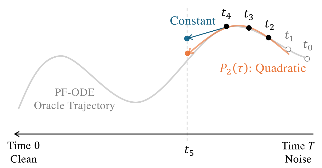
A degree-\(n\) update needs \(n{+}1\) anchors. When they are available (sufficient history, \(i \ge n{+}1\)), we use the full degree-\(n\) scheme. During the initial steps (insufficient history, \(i \le n\)), we use the highest feasible degree, \(i{-}1\), and increase it as more anchors become available. We treat these two cases below.
Case I: \(i = n+1,\dots,M\) (Sufficient History).
With sufficient history, DEIS reuses the last \(n{+}1\) model evaluations as anchors, \[(\tau_j,{\mathbf{Y}}_j) := \bigl(t_{i-1-j}, \bm{\epsilon}_{\bm{\phi}^\times}(\tilde{{\mathbf{x}}}_{t_{i-1-j}},t_{i-1-j})\bigr), \quad j=0,\dots,n.\] Viewing \(\tau\mapsto\bm{\epsilon}_{\bm{\phi}^\times}({\mathbf{x}}_\tau,\tau)\) as a smooth function along the trajectory, we construct the degree-\(n\) Lagrange polynomial \[P_n(\tau) = \sum_{j=0}^{n} \underbrace{\Bigl[\prod_{\substack{k=0\\ k\neq j}}^{n} \frac{\tau - t_{i-1-k}}{\,t_{i-1-j} - t_{i-1-k}\,}\Bigr]}_{=:~\ell_j^{(i)}(\tau)} \bm{\epsilon}_{\bm{\phi}^\times}\bigl(\tilde{\mathbf x}_{t_{i-1-j}}, t_{i-1-j}\bigr)\] which by construction satisfies \(P_n(\tau_j)={\mathbf{Y}}_j\) for each anchor: \[P_n\bigl(\tau_j\bigr) = {\mathbf{Y}}_j = \bm{\epsilon}_{\bm{\phi}^\times}\bigl(\tilde{\mathbf x}_{t_{i-1-j}}, t_{i-1-j}\bigr), \quad j=0,\ldots,n.\] Each \(\ell_j^{(i)}\) satisfies \[\ell_j^{(i)}\bigl(t_{i-1-m}\bigr) = \begin{cases} 1,&m=j,\\ 0,&m\neq j. \end{cases}\]
The polynomial is then extrapolated beyond the most recent anchor \(t_{i-1}\) over the new step: \[\bm{\epsilon}_{\bm{\phi}^\times}({\mathbf{x}}_\tau,\tau) \approx P_n(\tau)=\sum_{j=0}^{n}\ell_j^{(i)}(\tau) \bm{\epsilon}_{\bm{\phi}^\times}\bigl(\tilde{{\mathbf{x}}}_{t_{i-1-j}}, t_{i-1-j}\bigr), \quad \tau \in [t_i,t_{i-1}].\] We then substitute \(P_n(\tau)\) for \({\bm{\epsilon}}_{\bm{\phi}^\times}({\mathbf{x}}_\tau,\tau)\) in the exponential–integrator formula (Equation \(\eqref{eq:variation_of_constants}\)): \[\begin{align*} \int_{t_{i-1}}^{t_i} \frac{g^2(\tau)}{2\sigma_\tau} \mathcal{E}(\tau\to t_i) {\bm{\epsilon}}_{\bm{\phi}^\times}({\mathbf{x}}_\tau,\tau)\mathop{}\!\mathrm{d}\tau &\approx \sum_{j=0}^{n} \underbrace{ \int_{t_{i-1}}^{t_i} \frac{g^2(\tau)}{2\sigma_\tau} \mathcal{E}(\tau\to t_i) \ell_j^{(i)}(\tau)\mathop{}\!\mathrm{d}\tau }_{=:~C_{i,j}} \\ &\qquad\cdot {\bm{\epsilon}}_{\bm{\phi}^\times} (\tilde{\mathbf{x}}_{t_{i-1-j}},t_{i-1-j}). \end{align*}\] The coefficients \[C_{i,j} := \frac{1}{2} \int_{t_{i-1}}^{t_i} \frac{g^2(\tau)}{\sigma_\tau} \mathcal{E}(\tau\to t_i) \ell_j^{(i)}(\tau)\mathop{}\!\mathrm{d}\tau\] depend only on the noise schedule and the chosen time grid and can therefore be precomputed. For schedules admitting suitable antiderivatives, these coefficients are available in closed form; otherwise they can be evaluated numerically to high accuracy.
Integrating the linear part exactly with \(\mathcal{E}(t_{i-1}\to t_i)\) gives the AB-DEIS-\(n\) update \[\tilde{\mathbf{x}}_{t_i} = \mathcal{E}(t_{i-1}\to t_i)\tilde{\mathbf{x}}_{t_{i-1}} + \sum_{j=0}^{n} C_{i,j} {\bm{\epsilon}}_{\bm{\phi}^\times} (\tilde{\mathbf{x}}_{t_{i-1-j}},t_{i-1-j}).\] For the local truncation statements below, let \(h\) denote a characteristic local step size and assume neighboring step ratios remain bounded. Under standard smoothness assumptions on the model prediction along the empirical trajectory and regularity of the schedule-dependent weight, the full-history degree-\(n\) construction has formal order \(n+1\), with one-step local defect \(\mathcal O(h^{n+2})\).
Case II: \(i=1,\dots,n\) (Insufficient History).
During the initial steps, only \(i\) past model evaluations are available. We therefore use all available anchors and set the polynomial degree to \(i{-}1\): \[P_{i-1}(\tau) = \sum_{j=0}^{i-1} \ell_j^{(i)}(\tau) \bm{\epsilon}_{\bm{\phi}^\times}\bigl(\tilde{\mathbf x}_{t_{i-1-j}}, t_{i-1-j}\bigr),\] where \(\ell_j^{(i)}\) is the Lagrange basis of degree \(i{-}1\) built on the nodes at time \(\{t_{i-1}, t_{i-2},\ldots,t_{0}\}\). This matches all available anchors and transitions into the full-history formula once \(i\ge n{+}1\).
This is the standard warm-start situation for a multistep method. The first step uses a constant approximation, the second uses a linear extrapolation, the third uses a quadratic extrapolation, and so on, until the target degree \(n\) becomes available.
Example: Special Cases of Lagrange Polynomials
Degree \(0\) (one anchor): \[P_0(\tau) = \bm{\epsilon}_{\bm{\phi}^\times}(\tilde{\mathbf{x}}_{t_{i-1}}, t_{i-1}).\] This holds the neural prediction fixed at its start-of-step value, exactly as in the first-order DDIM approximation.
Degree \(1\) (two anchors): the Lagrange polynomial is a linear map passing through the two pre-specified anchors. \[P_1(\tau) = \underbrace{\frac{\tau - t_{i-2}}{t_{i-1} - t_{i-2}}}_{\displaystyle \ell_{i-1}(\tau)} \,\bm{\epsilon}_{\bm{\phi}^\times}(\tilde{\mathbf{x}}_{t_{i-1}}, t_{i-1}) + \underbrace{\frac{\tau - t_{i-1}}{t_{i-2} - t_{i-1}}}_{\displaystyle \ell_{i-2}(\tau)} \,\bm{\epsilon}_{\bm{\phi}^\times}(\tilde{\mathbf{x}}_{t_{i-2}}, t_{i-2}).\] Here \(\ell_{i-1}(\tau)\) and \(\ell_{i-2}(\tau)\) are the Lagrange basis weights. They satisfy the interpolation conditions \(P_1(t_{i-1})=\bm{\epsilon}_{\bm{\phi}^\times}(\tilde{\mathbf{x}}_{t_{i-1}}, t_{i-1})\) and \(P_1(t_{i-2})=\bm{\epsilon}_{\bm{\phi}^\times}(\tilde{\mathbf{x}}_{t_{i-2}}, t_{i-2})\), with \(\ell_{i-1}(\tau)+\ell_{i-2}(\tau)=1\).
Summary of AB-DEIS-\(n\) Update.
Combining the sufficient-history and warm-start cases gives the AB-DEIS-\(n\) update7 Here, \(n\) is the target polynomial degree, using up to \(n{+}1\) past evaluations:
\[\begin{align*} \tilde{\mathbf{x}}_{t_i} = \mathcal{E}(t_{i-1} \to t_i)\,\tilde{\mathbf{x}}_{t_{i-1}} + \sum_{j=0}^{\min\{n,\, i-1\}} C_{i,j}\,{\bm{\epsilon}}_{\bm{\phi}^\times}(\tilde{\mathbf{x}}_{t_{i-1-j}},\,t_{i-1-j}), \end{align*}\] with coefficients \[\begin{align*} C_{i,j} := \frac{1}{2} \int_{t_{i-1}}^{t_i} \frac{g^2(\tau)}{\sigma_\tau}\,\mathcal{E}(\tau \to t_i)\, \Bigg[\prod_{\substack{k=0\\ k\neq j}}^{\min\{n,\, i-1\}} \frac{\tau - t_{i-1-k}}{\,t_{i-1-j} - t_{i-1-k}\,}\Bigg]\,d\tau. \end{align*}\]
When \(i\ge n{+}1\) (sufficient history), \(\min\{n,\,i-1\}=n\), and the full-history degree-\(n\) step has one-step local truncation error \(\mathcal O(h^{n+2})\) under the assumptions above, corresponding to a method of order \(n+1\).
During warm start (\(i\le n\)), the degree is \(i-1\), so the one-step local truncation error is \(\mathcal O(h^{i+1})\), and the corresponding step is formally of order \(i\). Thus, the order increases from \(1\) at the first step and reaches the full order \(n+1\) once \(n+1\) anchors are available. As with standard multistep methods, lower-order warm-start steps do not by themselves establish a global order-\((n+1)\) guarantee; such a guarantee also requires stability and starting values of sufficient accuracy.
Very large \(n\) can degrade numerical behavior because high-degree extrapolation becomes increasingly sensitive to the spacing of the anchors, errors in the stored model predictions, and stability considerations. Relatively small polynomial degrees are therefore preferred in practice.
As we will see in the following subsection, the special case \(n{=}0\) reduces exactly to deterministic DDIM, i.e., the first-order factored exponential-integrator update.
DDIM = AB-DEIS-0
The connection to DDIM becomes immediate at degree \(n=0\). In this case, the Lagrange polynomial is constant, so DEIS uses only the most recent model prediction throughout the next step. The corresponding coefficient simplifies to \[C_{i0} = \frac{1}{2} \int_{t_{i-1}}^{t_{i}} \frac{g^2(\tau)}{\sigma_\tau} \mathcal{E}(\tau \rightarrow t_i) \mathrm{d}\tau.\] Substituting into the update formula yields the zeroth-order AB-DEIS scheme: \[\begin{align} \label{eq:deis-0} \tilde{\mathbf{x}}_{t_{i}} &= \mathcal{E}(t_{i-1} \rightarrow t_{i})\tilde{\mathbf{x}}_{t_{i-1}} + C_{i0} \bm{\epsilon}_{\bm{\phi}^\times}(\tilde{\mathbf{x}}_{t_{i-1}}, t_{i-1})\nonumber\\ &=e^{\int_{t_{i-1}}^{t_{i}}f(u)\mathop{}\!\mathrm{d}u} \tilde{\mathbf{x}}_{t_{i-1}} + \Big( \int_{t_{i-1}}^{t_{i}} \frac{g^2(\tau)}{2\sigma_\tau} e^{\int_{\tau}^{t_{i}}f(u)\mathop{}\!\mathrm{d}u} \mathrm{d}\tau \Big) \bm{\epsilon}_{\bm{\phi}^\times}(\tilde{\mathbf{x}}_{t_{i-1}}, t_{i-1}). \end{align}\] This is exactly the same first-order factored approximation used by deterministic DDIM: the neural prediction is held fixed at \(t_{i-1}\), while the known integrating factor and schedule-dependent coefficient remain inside the integral and are propagated over the full step. Hence, AB-DEIS-0 and DDIM are not merely first-order equivalent; they give the same finite-step update.
Proposition: DDIM = AB-DEIS-0
Equation \(\eqref{eq:deis-0}\) is identical to the DDIM update in Equation \(\eqref{eq:ddim-euler}\).
This also clarifies the role of DEIS in the solver hierarchy. We remark that the index “\(0\)” refers to the polynomial degree, not the numerical order: AB-DEIS-0 is still a first-order method. Higher-degree DEIS keeps the same analytic treatment of the known diffusion dynamics but replaces this constant prediction by polynomial extrapolation from additional past model evaluations. Thus, DDIM is the degree-zero base case from which the DEIS multistep construction naturally extends.
Later, in Section 1.5.4, we will encounter
another route to a multistep diffusion solver; that is,
DPM-Solver++(2M). It starts from a local Taylor expansion
of the data prediction in log-SNR time and recycles previous model
evaluations through a backward finite difference to estimate the
required derivative. Although its representation and derivation differ
from those of DEIS, both methods use past model evaluations to capture
the variation of the neural prediction without introducing additional
within-step stages. We return to this connection in Section 1.5.5, where we compare the two
constructions more explicitly.
DPM-Solver
DPM-Solver (Lu et al.
2022a) develops higher-order solvers for the empirical PF-ODE by
exploiting the same diffusion-specific structure that appeared in our
discussion of DDIM. The central goal is to obtain accurate samples using
far fewer neural-network evaluations than a first-order sampler. The
original DPM-Solver focuses on noise prediction and constructs first-,
second-, and third-order single-step solvers; later extensions,
including DPM-Solver++ (Lu et al. 2022b) and DPM-Solver-v3 (Zheng et al. 2023),
further develop this family.
High-Level Idea of DPM-Solver.
The DDIM discussion in Section 1.2 showed that, under \({\bm{\epsilon}}\)-prediction, a first-order update can be obtained by retaining the known diffusion schedule analytically while holding the neural prediction fixed over each step, \[{\bm{\epsilon}}_{\bm{\phi}^\times}({\mathbf{x}}_\tau,\tau) \approx {\bm{\epsilon}}_{\bm{\phi}^\times}(\tilde{\mathbf{x}}_s,s).\] DPM-Solver (Lu et al. 2022a) builds naturally on this idea: rather than treating the neural prediction as constant, it seeks higher-order approximations of how the prediction varies along the trajectory. Like DEIS, it starts from the semilinear \({\bm{\epsilon}}\)-prediction form of the PF-ODE, \[\begin{align} \label{eq:noise-alpha-sigma} \frac{\mathop{}\!\mathrm{d}{\mathbf{x}}_t}{\mathop{}\!\mathrm{d}t} = \frac{\alpha_t'}{\alpha_t}{\mathbf{x}}_t - \sigma_t \left( \frac{\alpha_t'}{\alpha_t} - \frac{\sigma_t'}{\sigma_t} \right) {\bm{\epsilon}}_{{\bm{\phi}}^\times}({\mathbf{x}}_t,t), \end{align}\] and its variation-of-constants representation introduced in the Prologue. Its key additional ingredient is to reparameterize time by the half-log signal-to-noise ratio, following the log-SNR parameterization of VDM (Kingma et al. 2021), \[\begin{align} \label{eq:lambda} \lambda_t := \log\frac{\alpha_t}{\sigma_t}. \end{align}\] This coordinate is directly related to DDIM’s schedule-aligned clock \(\rho_t=\sigma_t/\alpha_t\) (discussed around Equation \(\eqref{eq:ddim-coordinate-ode-t}\)) through \(\rho_t=e^{-\lambda_t}\), and turns the remaining model-dependent term into a particularly convenient exponentially weighted integral. Local Taylor approximations of the neural prediction in \(\lambda\) can then be integrated analytically, providing a systematic route from the first-order DDIM update to higher-order diffusion solvers.
DPM-Solver’s Insight: Time Reparameterization via Log-SNR
We now make the log-SNR reparameterization in Equation \(\eqref{eq:lambda}\) precise and derive the corresponding PF-ODE representation.
Change-of-Variable to Log-SNR in PF-ODE.
Suppose that \(\alpha_t>0\), \(\sigma_t>0\), and the log-SNR coordinate \(\lambda_t\) in Equation \(\eqref{eq:lambda}\) is strictly monotone on the interval of interest. It then admits an inverse function \(t_\lambda(\cdot)\) satisfying \[t=t_\lambda(\lambda(t)).\] For schedules with \(\sigma_0=0\), one has \(\lambda_t\to+\infty\) as \(t\to0\), so formulas involving the endpoint \(t=0\) are understood through the corresponding limit or through a small positive terminal time in a numerical implementation.
We then express the state, schedule, and neural prediction in the \(\lambda\)-coordinate. A hat (\(\hat{\cdot}\)) together with \(\lambda\) indicates that the corresponding quantity is viewed in this reparameterized time coordinate. More precisely, define \[\begin{align} \begin{aligned} \label{eq:change-of-var-x-epsilon} \hat{{\mathbf{x}}}_{\lambda} &:= {\mathbf{x}}_{t_\lambda(\lambda)}, \\ \alpha_\lambda &:= \alpha_{t_\lambda(\lambda)}, \qquad \sigma_\lambda := \sigma_{t_\lambda(\lambda)}, \\ \hat{\bm{\epsilon}}_{\bm{\phi}^\times}({\mathbf{x}},\lambda) &:= \bm{\epsilon}_{\bm{\phi}^\times} \bigl( {\mathbf{x}}, t_\lambda(\lambda) \bigr). \end{aligned} \end{align}\] Hence, along the empirical PF-ODE trajectory, \[\hat{\bm{\epsilon}}_{\bm{\phi}^\times} (\hat{\mathbf{x}}_\lambda,\lambda) = \bm{\epsilon}_{\bm{\phi}^\times} \bigl( {\mathbf{x}}_{t_\lambda(\lambda)}, t_\lambda(\lambda) \bigr).\] Since \[\frac{\mathop{}\!\mathrm{d}\lambda_t}{\mathop{}\!\mathrm{d}t} = \frac{\alpha_t'}{\alpha_t} - \frac{\sigma_t'}{\sigma_t},\] the PF-ODE in Equation \(\eqref{eq:noise-alpha-sigma}\) can be written as \[\frac{\mathop{}\!\mathrm{d}{\mathbf{x}}_t}{\mathop{}\!\mathrm{d}t} = \frac{\mathop{}\!\mathrm{d}\log\alpha_t}{\mathop{}\!\mathrm{d}t}{\mathbf{x}}_t - \sigma_t \frac{\mathop{}\!\mathrm{d}\lambda_t}{\mathop{}\!\mathrm{d}t} \bm{\epsilon}_{\bm{\phi}^\times}({\mathbf{x}}_t,t).\] Applying the chain rule, \[\frac{\mathop{}\!\mathrm{d}{\mathbf{x}}_t}{\mathop{}\!\mathrm{d}t} = \frac{\mathop{}\!\mathrm{d}\hat{\mathbf{x}}_\lambda}{\mathop{}\!\mathrm{d}\lambda} \frac{\mathop{}\!\mathrm{d}\lambda_t}{\mathop{}\!\mathrm{d}t}, \qquad \frac{\mathop{}\!\mathrm{d}\log\alpha_t}{\mathop{}\!\mathrm{d}t} = \frac{\mathop{}\!\mathrm{d}\log\alpha_\lambda}{\mathop{}\!\mathrm{d}\lambda} \frac{\mathop{}\!\mathrm{d}\lambda_t}{\mathop{}\!\mathrm{d}t},\] gives the PF-ODE in log-SNR time:
\[\begin{align} \label{eq:diffusion_ode_lambda_eps} \frac{\mathop{}\!\mathrm{d}\hat{{\mathbf{x}}}_\lambda}{\mathop{}\!\mathrm{d}\lambda} = \frac{\mathop{}\!\mathrm{d}\log\alpha_\lambda}{\mathop{}\!\mathrm{d}\lambda} \hat{{\mathbf{x}}}_\lambda - \sigma_\lambda \hat{\bm{\epsilon}}_{\bm{\phi}^\times} (\hat{{\mathbf{x}}}_\lambda,\lambda). \end{align}\]
Applying the same exponential-integrator (variation-of-constants) technique to Equation \(\eqref{eq:diffusion_ode_lambda_eps}\) gives the following exact solution.
Proposition: Exponentially Weighted Exact Solution
Given an initial value \({\mathbf{x}}_s\) at time \(s>0\), the exact empirical PF-ODE solution \(\widetilde{\bm{\Psi}}_{s\to t}({\mathbf{x}}_s)\) at time \(t\in(0,s]\) can be re-expressed as \[\begin{equation} \label{eq:analytic_solution} \widetilde{\bm{\Psi}}_{s\to t}({\mathbf{x}}_s) = \frac{\alpha_t}{\alpha_s}{\mathbf{x}}_s - \alpha_t \int_{\lambda_s}^{\lambda_t} e^{-\lambda} \hat{\bm{\epsilon}}_{\bm{\phi}^\times} (\hat{\mathbf{x}}_\lambda,\lambda) \mathop{}\!\mathrm{d}\lambda. \end{equation}\] When the endpoint satisfies \(\sigma_0=0\), the case \(t=0\) is understood through the corresponding limit.
Proof for Proposition. From Equation \(\eqref{eq:diffusion_ode_lambda_eps}\), the integrating factor associated with the linear term satisfies \[\exp\left( \int_{\lambda_s}^{\lambda_t} \frac{\mathop{}\!\mathrm{d}\log\alpha_\lambda}{\mathop{}\!\mathrm{d}\lambda} \mathop{}\!\mathrm{d}\lambda \right) = \frac{\alpha_t}{\alpha_s}.\] Therefore, the variation-of-constants formula gives \[\begin{align*} \widetilde{\bm{\Psi}}_{s\to t}({\mathbf{x}}_s) &= \frac{\alpha_t}{\alpha_s}{\mathbf{x}}_s - \int_{\lambda_s}^{\lambda_t} \frac{\alpha_t}{\alpha_\lambda} \sigma_\lambda \hat{\bm{\epsilon}}_{\bm{\phi}^\times} (\hat{\mathbf{x}}_\lambda,\lambda) \mathop{}\!\mathrm{d}\lambda \\ &= \frac{\alpha_t}{\alpha_s}{\mathbf{x}}_s - \alpha_t \int_{\lambda_s}^{\lambda_t} e^{-\lambda} \hat{\bm{\epsilon}}_{\bm{\phi}^\times} (\hat{\mathbf{x}}_\lambda,\lambda) \mathop{}\!\mathrm{d}\lambda, \end{align*}\] where the last equality follows from \(\sigma_\lambda/\alpha_\lambda=e^{-\lambda}\). ■
The key numerical consequence is now explicit. In \(\lambda\)-time, the only model-dependent quantity in the exact solution appears inside \[\int_{\lambda_s}^{\lambda_t} e^{-\lambda} \hat{\bm{\epsilon}}_{\bm{\phi}^\times} (\hat{\mathbf{x}}_\lambda,\lambda)\mathop{}\!\mathrm{d}\lambda.\] When the model output is locally approximated by a Taylor polynomial in \(\lambda\), the resulting exponentially weighted polynomial terms can be integrated in closed form, yielding explicit higher-order update coefficients. Thus, as in the factored viewpoint of the Prologue, the known schedule dependence is retained analytically while the approximation is concentrated on the neural prediction.
Intuition of Why Reparameterize Time?
For strictly monotone \(\lambda(t)\), a local first-order change of variables gives \[|\Delta t| \approx \frac{|\Delta\lambda|}{|\lambda'(t)|}.\] Thus, if the numerical grid uses a fixed step size \(|\Delta\lambda|\), the induced step in \(t\) is smaller where \(|\lambda'(t)|\) is larger (i.e., where \(\lambda\) changes rapidly with \(t\)), and larger where \(|\lambda'(t)|\) is smaller.
The reparameterization itself does not alter the PF-ODE solution path; it only changes how the same path is parameterized: \[\frac{\mathop{}\!\mathrm{d}\hat{\mathbf{x}}_\lambda}{\mathop{}\!\mathrm{d}\lambda} = \frac{1}{\lambda'(t)} \frac{\mathop{}\!\mathrm{d}{\mathbf{x}}_t}{\mathop{}\!\mathrm{d}t}.\] Hence, where \(|\lambda'(t)|\) is large, the same change of the trajectory with respect to \(t\) is represented over a larger range of \(\lambda\).
More importantly, \(\lambda(t)\) measures progress through the diffusion process directly in terms of the relative balance between signal and noise. A fixed \(\Delta\lambda\) corresponds to a fixed multiplicative change in \(\alpha_t/\sigma_t\), or equivalently to a fixed additive change in log-SNR, whereas the same \(\Delta t\) may correspond to very different changes in corruption level at different times. Therefore, choosing numerical nodes uniformly in \(\lambda\) provides a natural way to redistribute resolution along the diffusion trajectory. The precise induced spacing in the original time variable \(t\) depends on the chosen noise schedule. Two simple examples illustrate this effect:
\((\alpha_t,\sigma_t)=(1-t,t)\). This corresponds to the linear interpolation commonly used in flow matching. Then \[\lambda(t) = \log\frac{1-t}{t}, \qquad \lambda'(t) = -\frac{1}{t(1-t)},\] so locally \[|\Delta t| \approx |\Delta\lambda|\,t(1-t).\] Hence, a uniform grid in \(\lambda\) induces very small steps in \(t\) near both endpoints \(t\to0\) and \(t\to1\), and larger steps around the middle of the trajectory.
\((\alpha_t,\sigma_t)=(1,t)\). This corresponds to the EDM parameterization (Karras et al. 2022) when the independent variable \(t\) is taken directly as the noise level \(\sigma_t\). Then \[\lambda(t) = \log\frac{1}{t}, \qquad \lambda'(t) = -\frac{1}{t},\] and therefore \[|\Delta t| \approx |\Delta\lambda|\,t.\] In fact, uniform spacing in \(\lambda\) implies \[t=e^{-\lambda},\] so the corresponding noise levels are geometrically spaced. Thus, the grid contains finer absolute spacing at small noise levels (high SNR) and coarser absolute spacing at large noise levels (low SNR).
Estimating the Integral with Taylor Expansion
DEIS and DPM-Solver exploit the same factored principle but obtain higher-order information in different ways. DEIS reuses predictions from previous completed steps to extrapolate the neural prediction over the next interval. DPM-Solver instead works in the log-SNR coordinate \(\lambda\) and uses a local Taylor expansion of the neural prediction, with the required higher-order information obtained from additional evaluations within the current step. We now derive this single-step construction.
From Equation \(\eqref{eq:analytic_solution}\), the exact empirical PF-ODE flow initialized at the current numerical state \(\tilde{\mathbf{x}}_s\) is \[\begin{equation} \label{eqn:analytic_solution_each_step} \widetilde{\bm{\Psi}}_{s\to t}(\tilde{\mathbf{x}}_s) = \frac{\alpha_t}{\alpha_s}\tilde{\mathbf{x}}_s - \alpha_t \int_{\lambda_s}^{\lambda_t} e^{-\lambda} \hat{\bm{\epsilon}}_{\bm{\phi}^\times} (\hat{\mathbf{x}}_\lambda,\lambda) \mathop{}\!\mathrm{d}\lambda, \end{equation}\] where \(\hat{\mathbf{x}}_{\lambda_s}=\tilde{\mathbf{x}}_s\) and \(\hat{\mathbf{x}}_\lambda\) denotes the corresponding exact empirical PF-ODE trajectory over the current step. Therefore, after the known schedule-dependent factors have been handled analytically, the remaining numerical problem is to approximate \[\lambda \longmapsto \hat{\bm{\epsilon}}_{\bm{\phi}^\times} (\hat{\mathbf{x}}_\lambda,\lambda)\] inside the weighted integral.
For \(n\geq1\), we expand this neural prediction about \(\lambda_s\): \[\begin{equation*} \hat{\bm{\epsilon}}_{\bm{\phi}^\times} (\hat{\mathbf{x}}_\lambda,\lambda) = \sum_{k=0}^{n-1} \frac{(\lambda-\lambda_s)^k}{k!} \hat{\bm{\epsilon}}_{\bm{\phi}^\times}^{(k)} (\hat{\mathbf{x}}_{\lambda_s},\lambda_s) + \mathcal O\bigl((\lambda-\lambda_s)^n\bigr), \end{equation*}\] where \[\hat{\bm{\epsilon}}_{\bm{\phi}^\times}^{(k)} (\hat{\mathbf{x}}_\lambda,\lambda) := \frac{\mathop{}\!\mathrm{d}^k}{\mathop{}\!\mathrm{d}\lambda^k} \hat{\bm{\epsilon}}_{\bm{\phi}^\times} (\hat{\mathbf{x}}_\lambda,\lambda)\] denotes the \(k\)-th total derivative along the empirical PF-ODE trajectory. In particular, \[\frac{\mathop{}\!\mathrm{d}}{\mathop{}\!\mathrm{d}\lambda} \hat{\bm{\epsilon}}_{\bm{\phi}^\times} (\hat{\mathbf{x}}_\lambda,\lambda) = \frac{\partial}{\partial\lambda} \hat{\bm{\epsilon}}_{\bm{\phi}^\times} (\hat{\mathbf{x}}_\lambda,\lambda) + J_{{\mathbf{x}}} \hat{\bm{\epsilon}}_{\bm{\phi}^\times} (\hat{\mathbf{x}}_\lambda,\lambda) \frac{\mathop{}\!\mathrm{d}\hat{\mathbf{x}}_\lambda}{\mathop{}\!\mathrm{d}\lambda},\] so the derivative includes both the explicit dependence on \(\lambda\) and the dependence through the evolving state.
Substituting the Taylor expansion into eqn:analytic_solution_each_step gives
\[\begin{equation} \label{eq:k-th-expansion} \widetilde{\bm{\Psi}}_{s\to t}(\tilde{\mathbf{x}}_s) = \frac{\alpha_t}{\alpha_s}\tilde{\mathbf{x}}_s - \alpha_t \sum_{k=0}^{n-1} {\color{cyan} \hat{\bm{\epsilon}}_{\bm{\phi}^\times}^{(k)} (\hat{\mathbf{x}}_{\lambda_s},\lambda_s)} \,{\color{orange}C_k} + \mathcal O(h^{n+1}), \end{equation}\] where \[h:=\lambda_t-\lambda_s, \qquad {\color{orange}C_k} := \int_{\lambda_s}^{\lambda_t} e^{-\lambda} \frac{(\lambda-\lambda_s)^k}{k!} \mathop{}\!\mathrm{d}\lambda.\] The coefficients \({\color{orange}C_k}\) depend only on the log-SNR interval and can be evaluated analytically.
If the required trajectory derivatives were available, dropping the \(\mathcal O(h^{n+1})\) remainder would give the corresponding formal \(n\)-th order update. DPM-Solver avoids explicitly differentiating the neural network by approximating these derivatives from additional model evaluations, as described in the next subsection.
Example: DPM-Solver-1
For \(n=1\), the exact empirical flow satisfies \[\widetilde{\bm{\Psi}}_{s\to t}(\tilde{\mathbf{x}}_s) = \frac{\alpha_t}{\alpha_s}\tilde{\mathbf{x}}_s - \sigma_t \left(e^h-1\right) \bm{\epsilon}_{\bm{\phi}^\times}(\tilde{\mathbf{x}}_s,s) + \mathcal O(h^2).\] Dropping the \(\mathcal O(h^2)\) remainder defines DPM-Solver-1: \[\begin{align} \label{eq:dpm-1} \tilde{\mathbf{x}}_t^{\mathrm{DPM\text{-}Solver\text{-}1}} := \frac{\alpha_t}{\alpha_s}\tilde{\mathbf{x}}_s - \sigma_t \left(e^h-1\right) \bm{\epsilon}_{\bm{\phi}^\times}(\tilde{\mathbf{x}}_s,s). \end{align}\] This finite-step update is exactly the deterministic DDIM update, as shown in Section 1.4.4.
DPM-Solver-\(n\) with \(n \geq 2\) requires evaluating the \(k^{\text{th}}\)-derivative \(\hat{\bm{\epsilon}}_{\bm{\phi}^\times}^{(k)}(\hat{\mathbf{x}}_\lambda, \lambda)\) for \(k \leq n-1\). However, directly computing higher-order derivatives is computationally expensive in practice. Lu et al. (2022a) also propose efficient approximation methods for these derivatives, which will be detailed in the next subsection.
Implementation of DPM-Solver-\(n\)
DPM-Solver-\(n\) with \(n \geq 2\).
In practice, implementing a higher-order DPM-Solver-\(n\) entails the following:
Precomputing the coefficients \({\color{orange}C_k}\);
Approximating the \(k^{\text{th}}\) derivative \(\hat{\bm{\epsilon}}_{\bm{\phi}^\times}^{(k)}(\hat{\mathbf{x}}_\lambda,\lambda)\) for \(k \leq n-1\) to circumvent the costly computation of exact higher-order derivatives—a challenge well-studied in the ODE literature (Hochbruck and Ostermann 2005; Luan 2021). One common strategy is finite difference approximation.
We now elaborate on the first two points.
Precomputing \({\color{orange}C_k}\).
Let \(s\) and \(t\) denote the start and end times, respectively, and define \(h:=\lambda_t-\lambda_s\). The Taylor expansion of the exact empirical PF-ODE flow takes the form \[\begin{equation} \label{eq:analytic_expansion} \widetilde{\bm{\Psi}}_{s\to t}({\mathbf{x}}_s) = \frac{\alpha_t}{\alpha_s}{\mathbf{x}}_s - \sigma_t \sum_{k=0}^{n-1} h^{k+1} \varphi_{k+1}(h) \hat{\bm{\epsilon}}_{\bm{\phi}^\times}^{(k)} (\hat{\mathbf{x}}_{\lambda_s},\lambda_s) + \mathcal O(h^{n+1}), \end{equation}\] where, for \(m\geq1\), \[\varphi_m(h) := \frac{ e^h-\sum_{j=0}^{m-1}\frac{h^j}{j!} }{ h^m }, \qquad \varphi_m(0):=\frac{1}{m!}.\] For the first three cases, \[\begin{align*} \varphi_1(h) &= \frac{e^h-1}{h}, & \varphi_2(h) &= \frac{e^h-h-1}{h^2}, & \varphi_3(h) &= \frac{e^h-\frac{h^2}{2}-h-1}{h^3}. \end{align*}\]
Example: Third-Order Expansion with Exact Derivatives
For \(n=3\), Equation \(\eqref{eq:analytic_expansion}\) becomes \[\begin{equation} \label{eq:example-dpm-solver-3-exact} \begin{aligned} \widetilde{\bm{\Psi}}_{s\to t}({\mathbf{x}}_s) = \frac{\alpha_t}{\alpha_s}{\mathbf{x}}_s &- \sigma_t \left(e^h-1\right) \hat{\bm{\epsilon}}_{\bm{\phi}^\times} (\hat{\mathbf{x}}_{\lambda_s},\lambda_s) \\ &- \sigma_t \left(e^h-h-1\right) \hat{\bm{\epsilon}}_{\bm{\phi}^\times}^{(1)} (\hat{\mathbf{x}}_{\lambda_s},\lambda_s) \\ &- \sigma_t \left( e^h-\frac{h^2}{2}-h-1 \right) \hat{\bm{\epsilon}}_{\bm{\phi}^\times}^{(2)} (\hat{\mathbf{x}}_{\lambda_s},\lambda_s) + \mathcal O(h^4). \end{aligned} \end{equation}\]
Approximating \(\hat{\bm{\epsilon}}_{\bm{\phi}^\times}^{(k)}(\hat{\mathbf{x}}_\lambda,\lambda)\) for \(k \leq n-1\).
For \(n \geq 2\), following the standard approach of single-step ODE solvers (Atkinson et al. 2009), Lu et al. (2022a) use additional model evaluations within the current step to approximate the higher-order derivatives. We illustrate this idea for \(n=2\).
Let \(\gamma\in(0,1]\) specify a stage point in the log-SNR interval \([\lambda_s,\lambda_t]\). Given an estimate \(\tilde{\mathbf{x}}_s\) at \(s\), define \[s^{\mathrm{mid}} = t_\lambda\left(\lambda_s+\gamma h\right), \qquad h:=\lambda_t-\lambda_s.\] For \(\gamma\in(0,1)\) this is an interior point, while \(\gamma=1\) corresponds to the endpoint \(t\). We first use a DPM-Solver-1 step to predict the state at this stage: \[{\mathbf{x}}^{\mathrm{mid}} = \frac{\alpha_{s^{\mathrm{mid}}}}{\alpha_s}\tilde{\mathbf{x}}_s - \sigma_{s^{\mathrm{mid}}} \left(e^{\gamma h}-1\right) \bm{\epsilon}_{\bm{\phi}^\times}(\tilde{\mathbf{x}}_s,s).\] The difference between the model predictions at the starting and stage points then provides a finite-difference approximation of the first total derivative along the trajectory: \[\hat{\bm{\epsilon}}_{\bm{\phi}^\times}^{(1)} (\hat{\mathbf{x}}_{\lambda_s},\lambda_s) \approx \frac{ \bm{\epsilon}_{\bm{\phi}^\times} ({\mathbf{x}}^{\mathrm{mid}},s^{\mathrm{mid}}) - \bm{\epsilon}_{\bm{\phi}^\times} (\tilde{\mathbf{x}}_s,s) }{ \gamma h }.\] Substituting this approximation into the second-order expansion gives \[\begin{align} \label{eq:dpm-solver-2-app} \begin{aligned} \widetilde{\bm{\Psi}}_{s\to t}(\tilde{\mathbf{x}}_s) = \frac{\alpha_t}{\alpha_s}\tilde{\mathbf{x}}_s &- \sigma_t \left(e^h-1\right) \bm{\epsilon}_{\bm{\phi}^\times}(\tilde{\mathbf{x}}_s,s) \\ &- \frac{\sigma_t}{\gamma h} \left(e^h-h-1\right) \left[ \bm{\epsilon}_{\bm{\phi}^\times} ({\mathbf{x}}^{\mathrm{mid}},s^{\mathrm{mid}}) - \bm{\epsilon}_{\bm{\phi}^\times} (\tilde{\mathbf{x}}_s,s) \right] + \mathcal O(h^3). \end{aligned} \end{align}\] Thus, dropping the \(\mathcal O(h^3)\) remainder yields a second-order single-step update.
For the midpoint choice \(\gamma=\tfrac12\), DPM-Solver-2 admits the simpler two-stage form in Algorithm (DPM-Solver-2 (with γ=1/2)). This update differs from Equation \(\eqref{eq:dpm-solver-2-app}\) only by \(\mathcal O(h^3)\) and therefore has the same second-order accuracy.
Algorithm: DPM-Solver-2 (with γ=1/2)
Input: initial value \({\mathbf{x}}_T\), time steps \(\{t_i\}_{i=0}^M\), model \({\bm{\epsilon}}_{\bm{\phi}^\times}\)
\(\tilde{\mathbf{x}}_{t_0}\gets{\mathbf{x}}_T\)
for \(i\gets 1\) to \(M\) do
\(h_i \gets \lambda_{t_i}-\lambda_{t_{i-1}}\)
\(s_i^{\mathrm{mid}} \gets t_\lambda\left( \tfrac{\lambda_{t_{i-1}}+\lambda_{t_i}}{2} \right)\)
\({\mathbf{x}}_i^{\mathrm{mid}} \gets \tfrac{\alpha_{s_i^{\mathrm{mid}}}}{\alpha_{t_{i-1}}} \tilde{\mathbf{x}}_{t_{i-1}} - \sigma_{s_i^{\mathrm{mid}}} \left(e^{h_i/2}-1\right) {\bm{\epsilon}}_{\bm{\phi}^\times} (\tilde{\mathbf{x}}_{t_{i-1}},t_{i-1})\)
\(\tilde{\mathbf{x}}_{t_i} \gets \tfrac{\alpha_{t_i}}{\alpha_{t_{i-1}}} \tilde{\mathbf{x}}_{t_{i-1}} - \sigma_{t_i} \left(e^{h_i}-1\right) {\bm{\epsilon}}_{\bm{\phi}^\times} ({\mathbf{x}}_i^{\mathrm{mid}},s_i^{\mathrm{mid}})\)
\(\tilde{\mathbf{x}}_{t_M}\)
Remark. The finite difference above approximates the total \(\lambda\)-derivative of the neural prediction along the empirical PF-ODE trajectory. Under standard smoothness assumptions, \[\frac{ \bm{\epsilon}_{\bm{\phi}^\times} ({\mathbf{x}}^{\mathrm{mid}},s^{\mathrm{mid}}) - \bm{\epsilon}_{\bm{\phi}^\times} (\tilde{\mathbf{x}}_s,s) }{ \gamma h } = \hat{\bm{\epsilon}}_{\bm{\phi}^\times}^{(1)} (\hat{\mathbf{x}}_{\lambda_s},\lambda_s) + \mathcal O(h).\] Here, the intermediate state is itself obtained by a first-order DPM-Solver-1 step, whose stage error is \(\mathcal O(h^2)\); under smoothness of the model, this does not change the \(\mathcal O(h)\) accuracy of the difference quotient.
In Equation \(\eqref{eq:dpm-solver-2-app}\), this derivative approximation is multiplied by \[e^h-h-1=\mathcal O(h^2),\] so its induced error is \(\mathcal O(h^3)\). Hence, the resulting method is second-order accurate for any fixed \(\gamma\in(0,1]\).
This single-step construction uses two model evaluations: one at \((\tilde{\mathbf{x}}_s,s)\) and one at the predicted stage \(({\mathbf{x}}^{\mathrm{mid}},s^{\mathrm{mid}})\). The choice of \(\gamma\) does not change the formal second-order accuracy, but it changes the stage location and the error constant. In particular, \(\gamma=\tfrac 12\) places the second evaluation at the midpoint of the log-SNR interval, giving the commonly used midpoint version of DPM-Solver-2.
Implementation Detail: Selection of Sampling Timesteps.
Since DPM-Solver constructs its local high-order approximation in log-SNR time \(\lambda\), a natural choice is to place the numerical nodes uniformly in \(\lambda\). For a finite terminal time \(t_M>0\), this gives \[\lambda_{t_i} = \lambda_{t_0} + \frac{i}{M} \left( \lambda_{t_M}-\lambda_{t_0} \right), \qquad i=0,\ldots,M.\] If \(\sigma_0=0\), then \(\lambda_0=+\infty\), so in practice one instead uses a finite terminal log-SNR corresponding to a small positive time, with the endpoint handled by the corresponding limiting or final denoising step.
Although the derivation is carried out in \(\lambda\)-space, the pre-trained model and schedule \((\alpha_t,\sigma_t)\) are usually parameterized by the original diffusion time \(t\). During sampling, each selected log-SNR node is therefore mapped back through \[t_i=t_\lambda(\lambda_{t_i})\] whenever the model is evaluated or the schedule coefficients are required; see, for example, Algorithm (DPM-Solver-2 (with γ=1/2)). Thus, \(\lambda\) serves as the numerical integration coordinate, while the sampler continues to evaluate the original pre-trained diffusion model at its corresponding time labels.
DDIM \(=\) DPM-Solver-1
The first-order DPM-Solver recovers DDIM exactly. Both methods start from an exact integral representation of the same noise-prediction PF-ODE and make the same approximation over one step: \[{\bm{\epsilon}}_{\bm{\phi}^\times}({\mathbf{x}}_\tau,\tau) \approx {\bm{\epsilon}}_{\bm{\phi}^\times}(\tilde{\mathbf{x}}_s,s).\] The remaining schedule-dependent terms are then integrated analytically. DDIM applies this construction directly in the schedule-aligned form derived earlier, whereas DPM-Solver first rewrites the integral using the log-SNR coordinate \[\lambda_t = \log\frac{\alpha_t}{\sigma_t}.\] At first order, this change of numerical clock does not alter the constant approximation of the model prediction. Consequently, the two derivations produce exactly the same finite-step update.
Proposition: DDIM is DPM-Solver-1
For a fixed diffusion schedule \((\alpha_t,\sigma_t)\), the deterministic DDIM update in Equation \(\eqref{eq:ddim-euler}\) is identical to the DPM-Solver-1 update in Equation \(\eqref{eq:dpm-1}\).
Proof for Proposition. By the definition of \(\lambda\), \[\frac{\sigma_s}{\alpha_s} = e^{-\lambda_s}, \qquad \frac{\sigma_t}{\alpha_t} = e^{-\lambda_t}.\] Let \[h = \lambda_t-\lambda_s.\] Then \[e^h = \frac{\alpha_t/\sigma_t}{\alpha_s/\sigma_s} = \frac{\alpha_t\sigma_s}{\sigma_t\alpha_s},\] and therefore \[-\sigma_t(e^h-1) = \sigma_t - \frac{\alpha_t}{\alpha_s}\sigma_s = \alpha_t \left( \frac{\sigma_t}{\alpha_t} - \frac{\sigma_s}{\alpha_s} \right).\] Substituting this identity into the DPM-Solver-1 update gives \[\tilde{\mathbf{x}}_t = \frac{\alpha_t}{\alpha_s}\tilde{\mathbf{x}}_s + \alpha_t \left( \frac{\sigma_t}{\alpha_t} - \frac{\sigma_s}{\alpha_s} \right) {\bm{\epsilon}}_{\bm{\phi}^\times}(\tilde{\mathbf{x}}_s,s),\] which is exactly the deterministic DDIM update in Equation \(\eqref{eq:ddim-euler}\). ■
Thus, DPM-Solver-1 and DDIM are two derivations of the same first-order finite-step update. The log-SNR coordinate becomes consequential beyond first order: higher-order DPM-Solvers use it to approximate how the noise prediction changes along the trajectory, rather than treating that prediction as constant over the whole step.
Relation of DPM-Solver to Runge-Kutta-Type Solvers
DPM-Solver-1 is exactly the DDIM update (Section 1.4.4), so its first-order behavior is already understood. The higher-order question is how DPM-Solver improves this one-evaluation update.
The connection is to Runge-Kutta (RK) methods. Euler uses only the vector field at the beginning of a step, whereas RK methods obtain additional information through stages, i.e., evaluations at states and times generated within the current step; see Appendix A. Higher-order DPM-Solvers follow the same principle: instead of holding one neural prediction fixed over the whole step, they introduce additional within-step model evaluations to capture its variation. The diffusion-specific difference is that the known schedule-dependent factors are retained analytically, while the staged approximation is applied only to the learned prediction.
DPM-Solver-2 versus Plain Midpoint RK2.
We first compare DPM-Solver-2 with classical midpoint RK2 applied directly to the complete noise-prediction PF-ODE in log-SNR time from Equation \(\eqref{eq:diffusion_ode_lambda_eps}\). For brevity, denote its complete right-hand side by \({\mathbf{F}}(\hat{\mathbf{x}}_\lambda,\lambda)\).
For the midpoint choice \(\gamma=\tfrac12\), let \[\lambda_{\mathrm{mid}} := \lambda_{s^{\mathrm{mid}}} = \lambda_s+\frac{h}{2}, \qquad \alpha_{\mathrm{mid}} := \alpha_{s^{\mathrm{mid}}}, \qquad \sigma_{\mathrm{mid}} := \sigma_{s^{\mathrm{mid}}},\] and abbreviate \[\hat{\bm{\epsilon}}_s := \hat{\bm{\epsilon}}_{\bm{\phi}^\times}(\tilde{\mathbf{x}}_s,\lambda_s) = {\bm{\epsilon}}_{\bm{\phi}^\times}(\tilde{\mathbf{x}}_s,s).\]
Classical midpoint RK2 gives \[{\mathbf{x}}_{\mathrm{mid}}^{\mathrm{RK}} = \tilde{\mathbf{x}}_s + \frac{h}{2} {\mathbf{F}}(\tilde{\mathbf{x}}_s,\lambda_s),\] followed by \[\tilde{\mathbf{x}}_t^{\mathrm{RK2}} = \tilde{\mathbf{x}}_s + h\, {\mathbf{F}} \left( {\mathbf{x}}_{\mathrm{mid}}^{\mathrm{RK}}, \lambda_{\mathrm{mid}} \right).\] Thus, plain RK2 applies its two-stage construction to the complete PF-ODE velocity, including both the known schedule-dependent terms and the neural prediction.
By contrast, midpoint DPM-Solver-2 in Algorithm (DPM-Solver-2 (with γ=1/2)) first constructs the stage \[{\mathbf{x}}_{\mathrm{mid}}^{\mathrm{DPM2}} = \frac{\alpha_{\mathrm{mid}}}{\alpha_s}\tilde{\mathbf{x}}_s - \sigma_{\mathrm{mid}} \left( e^{h/2}-1 \right) \hat{\bm{\epsilon}}_s.\] Denoting the corresponding midpoint prediction by \[\hat{\bm{\epsilon}}_{\mathrm{mid}}^{\mathrm{DPM2}} := \hat{\bm{\epsilon}}_{\bm{\phi}^\times} \left( {\mathbf{x}}_{\mathrm{mid}}^{\mathrm{DPM2}}, \lambda_{\mathrm{mid}} \right),\] the full update is \[\tilde{\mathbf{x}}_t^{\mathrm{DPM2}} = \frac{\alpha_t}{\alpha_s}\tilde{\mathbf{x}}_s - \sigma_t \left( e^h-1 \right) \hat{\bm{\epsilon}}_{\mathrm{mid}}^{\mathrm{DPM2}}.\]
The structural difference is immediate. Plain midpoint RK2 discretizes the complete PF-ODE velocity, whereas DPM-Solver-2 retains the known diffusion-dependent evolution analytically and uses its two model evaluations only to approximate the variation of the noise prediction.
Under standard smoothness assumptions, both are second-order methods for the same empirical PF-ODE in \(\lambda\)-time. Their intermediate states generally differ by \(\mathcal O(h^2)\), and their complete one-step updates therefore satisfy \[\tilde{\mathbf{x}}_t^{\mathrm{DPM2}} - \tilde{\mathbf{x}}_t^{\mathrm{RK2}} = \mathcal O(h^3).\] Thus, DPM-Solver-2 follows the same two-stage midpoint principle as classical RK2, while exploiting the known diffusion structure before applying the numerical approximation.
DPM-Solver-2 versus Exponential Midpoint RK2.
A closer comparison keeps the semilinear decomposition in Equation \(\eqref{eq:diffusion_ode_lambda_eps}\) explicit and treats its known linear part analytically. The corresponding exponential midpoint RK2 construction first takes an exponential-Euler stage to the midpoint: \[{\mathbf{x}}_{\mathrm{mid}}^{\mathrm{ExpRK}} = \frac{\alpha_{\mathrm{mid}}}{\alpha_s}\tilde{\mathbf{x}}_s - \alpha_{\mathrm{mid}}\sigma_s \left[ \int_{\lambda_s}^{\lambda_{\mathrm{mid}}} \frac{1}{\alpha_\lambda}\mathop{}\!\mathrm{d}\lambda \right] \hat{\bm{\epsilon}}_s.\] After evaluating \[\hat{\bm{\epsilon}}_{\mathrm{mid}}^{\mathrm{ExpRK}} := \hat{\bm{\epsilon}}_{\bm{\phi}^\times} \left( {\mathbf{x}}_{\mathrm{mid}}^{\mathrm{ExpRK}}, \lambda_{\mathrm{mid}} \right),\] the full exponential-midpoint update is \[\tilde{\mathbf{x}}_t^{\mathrm{ExpRK2}} = \frac{\alpha_t}{\alpha_s}\tilde{\mathbf{x}}_s - \alpha_t\sigma_{\mathrm{mid}} \left[ \int_{\lambda_s}^{\lambda_t} \frac{1}{\alpha_\lambda}\mathop{}\!\mathrm{d}\lambda \right] \hat{\bm{\epsilon}}_{\mathrm{mid}}^{\mathrm{ExpRK}}.\] When the linear coefficient is constant, these integral coefficients reduce to the usual \(\varphi_1\) coefficients of explicit exponential midpoint RK2.
DPM-Solver-2 uses the same midpoint staging principle, but exploits the finer noise-prediction factorization \[-\sigma_\lambda \hat{\bm{\epsilon}}_{\bm{\phi}^\times}(\hat{\mathbf{x}}_\lambda,\lambda).\] Since \(\sigma_\lambda\) is also known from the diffusion schedule, DPM-Solver-2 retains it inside the integral and stages only the neural prediction. Its midpoint and full-step coefficients are therefore \[\alpha_{\mathrm{mid}} \int_{\lambda_s}^{\lambda_{\mathrm{mid}}} \frac{\sigma_\lambda}{\alpha_\lambda}\mathop{}\!\mathrm{d}\lambda = \sigma_{\mathrm{mid}} \left(e^{h/2}-1\right), \quad \text{and}\quad \alpha_t \int_{\lambda_s}^{\lambda_t} \frac{\sigma_\lambda}{\alpha_\lambda}\mathop{}\!\mathrm{d}\lambda = \sigma_t \left(e^h-1\right),\] respectively, recovering the update in Algorithm (DPM-Solver-2 (with γ=1/2)).
Hence, the three constructions differ in what is approximated by the RK stages: \[\begin{array}{rl} \mathbf{Plain RK2:} & \text{stage the complete PF-ODE velocity}, \\[4pt] \mathbf{ExpRK2:} & \begin{aligned}[t] &\text{propagate the linear part exactly;}\\ &\text{stage the coefficient-weighted residual } \sigma_\lambda\hat{\bm{\epsilon}}_{\bm{\phi}^\times}, \end{aligned} \\[6pt] \mathbf{DPM-Solver-2:} & \text{also retain }\sigma_\lambda\text{ analytically and stage only } \hat{\bm{\epsilon}}_{\bm{\phi}^\times}. \end{array}\]
The exponential-RK and DPM midpoint stages differ by \[{\mathbf{x}}_{\mathrm{mid}}^{\mathrm{DPM2}} - {\mathbf{x}}_{\mathrm{mid}}^{\mathrm{ExpRK}} = - \alpha_{\mathrm{mid}} \left[ \int_{\lambda_s}^{\lambda_{\mathrm{mid}}} \frac{\sigma_\lambda-\sigma_s}{\alpha_\lambda} \mathop{}\!\mathrm{d}\lambda \right] \hat{\bm{\epsilon}}_s = \mathcal O(h^2).\] For the complete step, a Taylor expansion about \(\lambda_{\mathrm{mid}}\) gives \[\int_{\lambda_s}^{\lambda_t} \frac{\sigma_\lambda-\sigma_{\mathrm{mid}}}{\alpha_\lambda} \mathop{}\!\mathrm{d}\lambda = \mathcal O(h^3),\] while smoothness of the neural prediction gives \[\hat{\bm{\epsilon}}_{\mathrm{mid}}^{\mathrm{DPM2}} - \hat{\bm{\epsilon}}_{\mathrm{mid}}^{\mathrm{ExpRK}} = \mathcal O(h^2).\] Consequently, \[\tilde{\mathbf{x}}_t^{\mathrm{DPM2}} - \tilde{\mathbf{x}}_t^{\mathrm{ExpRK2}} = \mathcal O(h^3).\] Thus, DPM-Solver-2 and exponential midpoint RK2 agree through second order, but DPM-Solver-2 retains one additional analytically known quantity, \(\sigma_\lambda\), inside the weighted integral.
Remark. The discussion above concerns the noise-prediction formulation in which DPM-Solver is derived. If a pre-trained model uses another prediction parameterization, its output may be converted pointwise to noise prediction through Equation in Chapter 6 at each stage. Just like the DDIM-case in Section 1.2.2, this should not be confused with directly applying a classical RK method to the raw prediction field: pointwise conversion and finite-step discretization are separate operations.
DPM-Solver and Runge–Kutta Methods
DPM-Solver combines the within-step staging principle of Runge–Kutta methods with the analytic treatment of known diffusion dynamics. DPM-Solver-1 is exactly DDIM, while higher-order DPM-Solvers use additional within-step evaluations to capture the variation of the neural prediction. The connection to classical RK methods is structural rather than an equality of finite-step formulas: DPM-Solver retains the known diffusion-dependent weights analytically before approximating the learned prediction.
DPM-Solver++
From
DPM-Solver to DPM-Solver++ for Guided Sampling
DPM-Solver++ (Lu et al. 2022b) was developed to
improve high-order sampling under strong guidance. In this regime, two
practical difficulties arise. First, large guidance scales can amplify
the model output and its derivatives, narrowing the convergence region
of high-order solvers and requiring smaller numerical steps. Second, the
guided prediction may drive the final solution outside the range
represented by the training data, leading to the train–test mismatch
discussed in Chapter 8.
DPM-Solver++ addresses these issues in two complementary
ways. It reformulates the diffusion ODE using data prediction, for which
data-space corrections such as dynamic thresholding can be applied, and
it develops a multistep variant that reuses previous model evaluations
to obtain smaller effective step sizes under a fixed NFE budget. We
first derive the data-prediction formulation and then introduce its
single-step and multistep second-order solvers.
DPM-Solver++’s
Methodology
DPM-Solver++ keeps the log-SNR coordinate \(\lambda\) introduced for DPM-Solver, but
expresses the empirical PF-ODE through data prediction rather than noise
prediction. Recall from Equation in Chapter 6
that \[{\bm{\epsilon}}_{\bm{\phi}^\times}({\mathbf{x}}_t,t)
=
\frac{
{\mathbf{x}}_t-\alpha_t{\mathbf{x}}_{\bm{\phi}^\times}({\mathbf{x}}_t,t)
}{
\sigma_t
}.\] Substituting this relation into the noise-prediction exact
solution in Equation \(\eqref{eq:analytic_solution}\) gives the
equivalent data-prediction form \[\begin{equation}
\label{eq:dpmpp-data-exact}
\widetilde{\bm{\Psi}}_{s\to t}({\mathbf{x}}_s)
=
\frac{\sigma_t}{\sigma_s}{\mathbf{x}}_s
+
\sigma_t
\int_{\lambda_s}^{\lambda_t}
e^\lambda
\hat{{\mathbf{x}}}_{\bm{\phi}^\times}
(\hat{\mathbf{x}}_\lambda,\lambda)
\mathop{}\!\mathrm{d}\lambda,
\end{equation}\] where, following Equation \(\eqref{eq:change-of-var-x-epsilon}\), we
define the \(\lambda\)-parameterized
data-prediction field by \[\hat{{\mathbf{x}}}_{\bm{\phi}^\times}
({\mathbf{x}},\lambda)
:=
{\mathbf{x}}_{\bm{\phi}^\times}
\bigl(
{\mathbf{x}},
t_\lambda(\lambda)
\bigr).\] Hence, along the empirical PF-ODE trajectory, \[\hat{{\mathbf{x}}}_{\bm{\phi}^\times}
(\hat{\mathbf{x}}_\lambda,\lambda)
=
{\mathbf{x}}_{\bm{\phi}^\times}
\bigl(
{\mathbf{x}}_{t_\lambda(\lambda)},
t_\lambda(\lambda)
\bigr).\]
Thus, the structure is exactly dual to DPM-Solver: the known
schedule-dependent evolution is handled analytically, while the only
model-dependent quantity inside the remaining integral is now the data
prediction. DPM-Solver++ develops two second-order
realizations of this exact form:
Single-Step Solver, DPM-Solver
++(2S). Use an additional model evaluation at an intermediate stage within the current step, analogous to the staged construction of DPM-Solver-2.Multistep Solver, DPM-Solver
++(2M). Reuse data predictions from the previous two completed steps. After the warm start, only one new model evaluation is required per step.
Remark. Without thresholding, converting a model output to data prediction is a pointwise algebraic re-expression of the same empirical PF-ODE. The numerical method can nevertheless change because the finite-step approximation is now applied to the data prediction rather than to the noise prediction. If thresholding is used, it is an additional modification of the model output and should be viewed separately from the numerical-order analysis below.
DPM-Solver++
Single-Step by Taylor Expansion
Following the DPM-Solver construction in Section 1.4.2,
DPM-Solver++ approximates the data prediction along the
empirical trajectory by a local Taylor expansion in log-SNR time. For
\(k\geq0\), denote its \(k\)-th total derivative along the empirical
PF-ODE trajectory by \[\hat{{\mathbf{x}}}_{\bm{\phi}^\times}^{(k)}
(\hat{\mathbf{x}}_\lambda,\lambda)
:=
\frac{\mathop{}\!\mathrm{d}^k}{\mathop{}\!\mathrm{d}\lambda^k}
\hat{{\mathbf{x}}}_{\bm{\phi}^\times}
(\hat{\mathbf{x}}_\lambda,\lambda).\]
For one step from \(t_{i-1}\) to \(t_i\), let \(h_i := \lambda_{t_i}-\lambda_{t_{i-1}} >0\). A Taylor expansion about \(\lambda_{t_{i-1}}\) gives \[\hat{{\mathbf{x}}}_{\bm{\phi}^\times} (\hat{\mathbf{x}}_\lambda,\lambda) = \sum_{k=0}^{n-1} \frac{ (\lambda-\lambda_{t_{i-1}})^k }{ k! } \hat{{\mathbf{x}}}_{\bm{\phi}^\times}^{(k)} \bigl( \hat{\mathbf{x}}_{\lambda_{t_{i-1}}}, \lambda_{t_{i-1}} \bigr) + \mathcal O \bigl( (\lambda-\lambda_{t_{i-1}})^n \bigr).\] Substituting this expansion into Equation \(\eqref{eq:dpmpp-data-exact}\) yields \[\begin{align} \label{eq:dpmpp-taylor-expansion} \widetilde{\bm{\Psi}}_{t_{i-1}\to t_i} (\tilde{\mathbf{x}}_{t_{i-1}}) = \frac{\sigma_{t_i}}{\sigma_{t_{i-1}}} \tilde{\mathbf{x}}_{t_{i-1}} + \alpha_{t_i} \sum_{k=0}^{n-1} h_i^{k+1} \varphi_{k+1}(-h_i) \hat{{\mathbf{x}}}_{\bm{\phi}^\times}^{(k)} \bigl( \hat{\mathbf{x}}_{\lambda_{t_{i-1}}}, \lambda_{t_{i-1}} \bigr) + \mathcal O(h_i^{n+1}), \end{align}\] where \(\varphi_m\) is defined in Equation \(\eqref{eq:analytic_expansion}\). Here we used \[\int_{\lambda_{t_{i-1}}}^{\lambda_{t_i}} e^\lambda \frac{ (\lambda-\lambda_{t_{i-1}})^k }{ k! } \mathop{}\!\mathrm{d}\lambda = e^{\lambda_{t_i}} h_i^{k+1} \varphi_{k+1}(-h_i),\] together with \(\sigma_{t_i}e^{\lambda_{t_i}}=\alpha_{t_i}\).
For \(n=1\), dropping the \(\mathcal O(h_i^2)\) remainder gives \[\tilde{\mathbf{x}}_{t_i} = \frac{\sigma_{t_i}}{\sigma_{t_{i-1}}} \tilde{\mathbf{x}}_{t_{i-1}} + \alpha_{t_i} \left( 1-e^{-h_i} \right) {\mathbf{D}}_{i-1}, \qquad {\mathbf{D}}_{i-1} := {\mathbf{x}}_{\bm{\phi}^\times} (\tilde{\mathbf{x}}_{t_{i-1}},t_{i-1}),\] which is exactly the deterministic DDIM update in data-prediction form.
For \(n=2\), the first total
derivative is approximated using an additional within-step stage. For
the midpoint choice, define \[s_i^{\mathrm{mid}}
:=
t_\lambda
\left(
\lambda_{t_{i-1}}+\frac{h_i}{2}
\right).\] A first-order DPM-Solver++ step predicts
the midpoint state \[{\mathbf{u}}_i
=
\frac{
\sigma_{s_i^{\mathrm{mid}}}
}{
\sigma_{t_{i-1}}
}
\tilde{\mathbf{x}}_{t_{i-1}}
+
\alpha_{s_i^{\mathrm{mid}}}
\left(
1-e^{-h_i/2}
\right)
{\mathbf{D}}_{i-1},\] at which we evaluate \[{\mathbf{D}}_i^{\mathrm{mid}}
:=
{\mathbf{x}}_{\bm{\phi}^\times}
({\mathbf{u}}_i,s_i^{\mathrm{mid}}).\] The midpoint
DPM-Solver++(2S) update then takes the particularly simple
form \[\tilde{\mathbf{x}}_{t_i}
=
\frac{\sigma_{t_i}}{\sigma_{t_{i-1}}}
\tilde{\mathbf{x}}_{t_{i-1}}
+
\alpha_{t_i}
\left(
1-e^{-h_i}
\right)
{\mathbf{D}}_i^{\mathrm{mid}}.\] As with midpoint DPM-Solver-2,
this simplified two-stage update differs from the direct second-order
Taylor/finite-difference construction only by \(\mathcal O(h_i^3)\) and therefore retains
second-order accuracy.
This yields the single-step DPM-Solver++ construction.
When \(n=1\), it reduces exactly to the
deterministic DDIM update in data-prediction form. When \(n=2\), approximating the first total \(\lambda\)-derivative using an additional
within-step model evaluation gives
DPM-Solver++(2S), the data-prediction counterpart
of DPM-Solver-2 in Algorithm (DPM-Solver-2 (with γ=1/2)). Its midpoint
implementation is summarized in Algorithm (DPM-Solver++(2S): a midpoint special case).
Algorithm: DPM-Solver++(2S): a midpoint special case
Input: initial value \({\mathbf{x}}_T\), time steps \(\{t_i\}_{i=0}^M\), data-prediction model \({\mathbf{x}}_{{\bm{\phi}}^\times}\)
\(\tilde{\mathbf{x}}_{t_0}\gets{\mathbf{x}}_T\)
\(\lambda_{t_i}\gets\log(\alpha_{t_i}/\sigma_{t_i})\) for \(i=0,\ldots,M\)
\({\mathbf{D}}_0 \gets {\mathbf{x}}_{{\bm{\phi}}^\times}(\tilde{\mathbf{x}}_{t_0},t_0)\) // cache start prediction
for \(i\gets 1\) to \(M\) do
\(h_i \gets \lambda_{t_i}-\lambda_{t_{i-1}}\)
\(s_i^{\mathrm{mid}} \gets t_\lambda \left( \tfrac{\lambda_{t_{i-1}}+\lambda_{t_i}}{2} \right)\)
\({\mathbf{u}}_i \gets \tfrac{\sigma_{s_i^{\mathrm{mid}}}}{\sigma_{t_{i-1}}} \tilde{\mathbf{x}}_{t_{i-1}} + \alpha_{s_i^{\mathrm{mid}}} \left( 1-e^{-h_i/2} \right) {\mathbf{D}}_{i-1}\) // predict midpoint stage
\({\mathbf{D}}_i^{\mathrm{mid}} \gets {\mathbf{x}}_{{\bm{\phi}}^\times} ({\mathbf{u}}_i,s_i^{\mathrm{mid}})\) // evaluate at midpoint
\(\tilde{\mathbf{x}}_{t_i} \gets \tfrac{\sigma_{t_i}}{\sigma_{t_{i-1}}} \tilde{\mathbf{x}}_{t_{i-1}} + \alpha_{t_i} \left( 1-e^{-h_i} \right) {\mathbf{D}}_i^{\mathrm{mid}}\)
if \(i<M\) then
\({\mathbf{D}}_i \gets {\mathbf{x}}_{{\bm{\phi}}^\times} (\tilde{\mathbf{x}}_{t_i},t_i)\) // cache for next step
\(\tilde{\mathbf{x}}_{t_M}\)
DPM-Solver++ Multistep
by Recycling History
DPM-Solver++(2S) obtains second-order information by
introducing an additional model evaluation within the current
step. DPM-Solver++(2M) takes a different route: it
reuses model predictions from previous completed steps to estimate the
same local variation. After initialization, this requires only one new
model evaluation per step, allowing more, and hence smaller, numerical
steps under the same NFE budget. This is particularly useful under
strong guidance, where large steps can reduce numerical stability.
The idea is simple. Recall that the second-order expansion in Equation \(\eqref{eq:dpmpp-taylor-expansion}\) requires both the current data prediction and its first total derivative with respect to \(\lambda\). The single-step method estimates this derivative using a new within-step stage; the multistep method instead estimates it from the recent history of model predictions.
For the first step, no such history is available, so we initialize with the first-order data-prediction update \[\tilde{\mathbf{x}}_{t_1} = \frac{\sigma_{t_1}}{\sigma_{t_0}} \tilde{\mathbf{x}}_{t_0} + \alpha_{t_1} \left( 1-e^{-h_1} \right) {\mathbf{D}}_0, \qquad {\mathbf{D}}_0 := {\mathbf{x}}_{\bm{\phi}^\times} (\tilde{\mathbf{x}}_{t_0},t_0).\] This is exactly the deterministic DDIM update in data-prediction form.
Once two completed-step predictions are available, for \(i\geq2\) define \[{\mathbf{D}}_{i-1} := {\mathbf{x}}_{\bm{\phi}^\times} (\tilde{\mathbf{x}}_{t_{i-1}},t_{i-1}), \qquad {\mathbf{D}}_{i-2} := {\mathbf{x}}_{\bm{\phi}^\times} (\tilde{\mathbf{x}}_{t_{i-2}},t_{i-2}).\] Keeping the first two terms of Equation \(\eqref{eq:dpmpp-taylor-expansion}\) gives \[\begin{align*} \widetilde{\bm{\Psi}}_{t_{i-1}\to t_i} (\tilde{\mathbf{x}}_{t_{i-1}}) = \frac{\sigma_{t_i}}{\sigma_{t_{i-1}}} \tilde{\mathbf{x}}_{t_{i-1}} &+ \alpha_{t_i} \left( 1-e^{-h_i} \right) {\mathbf{D}}_{i-1} \\ &+ \alpha_{t_i} \left( h_i-1+e^{-h_i} \right) \hat{{\mathbf{x}}}_{\bm{\phi}^\times}^{(1)} \bigl( \hat{\mathbf{x}}_{\lambda_{t_{i-1}}}, \lambda_{t_{i-1}} \bigr) + \mathcal O(h_i^3). \end{align*}\] Thus, the only additional quantity needed for a second-order update is the first total \(\lambda\)-derivative of the data prediction.
Instead of evaluating the model at a new intermediate stage,
DPM-Solver++(2M) estimates this derivative from the
previous completed step: \[\hat{{\mathbf{x}}}_{\bm{\phi}^\times}^{(1)}
\bigl(
\hat{\mathbf{x}}_{\lambda_{t_{i-1}}},
\lambda_{t_{i-1}}
\bigr)
\approx
\frac{
{\mathbf{D}}_{i-1}-{\mathbf{D}}_{i-2}
}{
h_{i-1}
}.\] Under standard smoothness assumptions, this backward
difference has error \(\mathcal
O(h_{i-1})\). Substituting it into the second-order expansion and
collecting the two prediction terms gives \[\tilde{\mathbf{x}}_{t_i}^{\mathrm{poly}}
=
\frac{\sigma_{t_i}}{\sigma_{t_{i-1}}}
\tilde{\mathbf{x}}_{t_{i-1}}
+
\alpha_{t_i}
\left(
1-e^{-h_i}
\right)
{\mathbf{D}}_i^{\mathrm{poly}},\] where \[{\mathbf{D}}_i^{\mathrm{poly}}
:=
{\mathbf{D}}_{i-1}
+
\frac{\beta(h_i)}{h_{i-1}}
\left(
{\mathbf{D}}_{i-1}-{\mathbf{D}}_{i-2}
\right),
\qquad
\beta(h)
:=
\frac{
h-1+e^{-h}
}{
1-e^{-h}
}.\] When consecutive step ratios remain bounded, this weighted
multistep update has one-step local defect \(\mathcal O(h_i^3)\).
The Practical
DPM-Solver++(2M) Update.
The expression above is already a valid second-order multistep
construction. DPM-Solver++(2M) uses a slightly simpler
coefficient that preserves the same order. Since \[\beta(h)
=
\frac{h}{2}
+
\frac{h^2}{12}
+
\mathcal O(h^3),\] define the step ratio \[r_i
:=
\frac{h_i}{h_{i-1}}\] and replace \({\mathbf{D}}_i^{\mathrm{poly}}\) by \[{\mathbf{D}}_i^{\mathrm{sim}}
:=
{\mathbf{D}}_{i-1}
+
\frac{r_i}{2}
\left(
{\mathbf{D}}_{i-1}-{\mathbf{D}}_{i-2}
\right).\] Equivalently, \[{\mathbf{D}}_i^{\mathrm{sim}}
=
\left(
1+\frac{r_i}{2}
\right){\mathbf{D}}_{i-1}
-
\frac{r_i}{2}{\mathbf{D}}_{i-2}.\] The interpretation is
straightforward: the two most recent model predictions tell us the local
direction in which the data prediction is changing, and \({\mathbf{D}}_i^{\mathrm{sim}}\)
extrapolates that trend into the current step.
Under the same smoothness and bounded-step-ratio assumptions, \[{\mathbf{D}}_i^{\mathrm{poly}}
-
{\mathbf{D}}_i^{\mathrm{sim}}
=
\mathcal O(h_i^2).\] Since \[\alpha_{t_i}
\left(
1-e^{-h_i}
\right)
=
\mathcal O(h_i),\] this simplification changes the state update
only by \(\mathcal O(h_i^3)\). Hence,
it preserves second-order accuracy, giving the practical
DPM-Solver++(2M) update
\[\tilde{\mathbf{x}}_{t_i} = \frac{\sigma_{t_i}}{\sigma_{t_{i-1}}} \tilde{\mathbf{x}}_{t_{i-1}} + \alpha_{t_i} \left( 1-e^{-h_i} \right) {\mathbf{D}}_i^{\mathrm{sim}}.\]
After computing \(\tilde{\mathbf{x}}_{t_i}\), the model is
evaluated once at the new state, \[{\mathbf{D}}_i
=
{\mathbf{x}}_{\bm{\phi}^\times}
(\tilde{\mathbf{x}}_{t_i},t_i),\] and this prediction is cached
for the next step. Thus, after the warm start, each
DPM-Solver++(2M) step requires only one new model
evaluation.
Remark. For uniform log-SNR steps, \(r_i=1\), so \[{\mathbf{D}}_i^{\mathrm{sim}}
=
\frac{3}{2}{\mathbf{D}}_{i-1}
-
\frac{1}{2}{\mathbf{D}}_{i-2}.\] The coefficients \((\frac 32,-\frac 12)\) are the familiar AB2
extrapolation weights for the model prediction. The complete
DPM-Solver++(2M) update is nevertheless not plain AB2: the
known diffusion-dependent factor \(\alpha_{t_i}(1-e^{-h_i})\) is retained
analytically.
The complete warm-start and two-step procedure is summarized in
Algorithm (DPM-Solver++(2M)). The key distinction
from DPM-Solver++(2S) is where the second-order information
comes from: 2S obtains it from an additional stage within the current
step, whereas 2M recycles model evaluations from previous completed
steps.
Algorithm: DPM-Solver++(2M)
Input: initial value \({\mathbf{x}}_T\), time steps \(\{t_i\}_{i=0}^M\), data-prediction model \({\mathbf{x}}_{{\bm{\phi}}^\times}\)
\(\tilde{\mathbf{x}}_{t_0}\gets{\mathbf{x}}_T\)
\(\lambda_{t_i}\gets\log(\alpha_{t_i}/\sigma_{t_i})\) for \(i=0,\ldots,M\)
\({\mathbf{D}}_0 \gets {\mathbf{x}}_{{\bm{\phi}}^\times} (\tilde{\mathbf{x}}_{t_0},t_0)\) // cache start prediction
Case I. Warm start (\(i=1\))
\(h_1 \gets \lambda_{t_1}-\lambda_{t_0}\)
\(\tilde{\mathbf{x}}_{t_1} \gets \tfrac{\sigma_{t_1}}{\sigma_{t_0}} \tilde{\mathbf{x}}_{t_0} + \alpha_{t_1} \left( 1-e^{-h_1} \right) {\mathbf{D}}_0\) // DDIM in data prediction
if \(M>1\) then
\({\mathbf{D}}_1 \gets {\mathbf{x}}_{{\bm{\phi}}^\times} (\tilde{\mathbf{x}}_{t_1},t_1)\) // cache for multistep update
Case II. Two-step multistep update (\(i\geq 2\))
for \(i\gets 2\) to \(M\) do
\(h_i \gets \lambda_{t_i}-\lambda_{t_{i-1}}\)
\(r_i \gets h_i/h_{i-1}\) // step ratio
\({\mathbf{D}}_i^{\mathrm{sim}} \gets \left( 1+\tfrac12 r_i \right) {\mathbf{D}}_{i-1} - \tfrac12 r_i {\mathbf{D}}_{i-2}\)
\(\tilde{\mathbf{x}}_{t_i} \gets \tfrac{\sigma_{t_i}}{\sigma_{t_{i-1}}} \tilde{\mathbf{x}}_{t_{i-1}} + \alpha_{t_i} \left( 1-e^{-h_i} \right) {\mathbf{D}}_i^{\mathrm{sim}}\)
if \(i<M\) then
\({\mathbf{D}}_i \gets {\mathbf{x}}_{{\bm{\phi}}^\times} (\tilde{\mathbf{x}}_{t_i},t_i)\) // one new model call; cache for next step
\(\tilde{\mathbf{x}}_{t_M}\)
Relation of DPM-Solver++(2M) to
DEIS
DPM-Solver++(2M) and DEIS use the same basic multistep
idea: reuse model predictions from previous completed steps to
approximate how the neural prediction changes over the next interval,
while keeping the known diffusion-dependent weights analytic. The
difference is the representation in which this idea is applied. DEIS was
formulated earlier using noise prediction in the original diffusion
time, whereas DPM-Solver++(2M) uses data prediction in
log-SNR time.
To expose the connection directly, we can apply the DEIS polynomial
extrapolation principle to the exact data-prediction integral underlying
DPM-Solver++. Recall that \[\widetilde{\bm{\Psi}}_{t_{i-1}\to t_i}
(\tilde{\mathbf{x}}_{t_{i-1}})
=
\frac{\sigma_{t_i}}{\sigma_{t_{i-1}}}
\tilde{\mathbf{x}}_{t_{i-1}}
+
\sigma_{t_i}
\int_{\lambda_{t_{i-1}}}^{\lambda_{t_i}}
e^\lambda
\hat{{\mathbf{x}}}_{\bm{\phi}^\times}
(\hat{\mathbf{x}}_\lambda,\lambda)
\mathop{}\!\mathrm{d}\lambda.\] The known weight \(e^\lambda\) is already handled
analytically. The only quantity that must be approximated over the step
is therefore the data prediction \[\lambda
\longmapsto
\hat{{\mathbf{x}}}_{\bm{\phi}^\times}
(\hat{\mathbf{x}}_\lambda,\lambda).\]
Using the two most recent cached predictions \({\mathbf{D}}_{i-2}\) and \({\mathbf{D}}_{i-1}\), the simplest nonconstant approximation is the unique affine polynomial through these two anchors. In Lagrange form, \[P_1(\lambda) = \frac{ \lambda-\lambda_{t_{i-2}} }{ h_{i-1} } {\mathbf{D}}_{i-1} - \frac{ \lambda-\lambda_{t_{i-1}} }{ h_{i-1} } {\mathbf{D}}_{i-2}.\] The same polynomial can be written more transparently around the most recent anchor as \[P_1(\lambda) = {\mathbf{D}}_{i-1} + \frac{ \lambda-\lambda_{t_{i-1}} }{ h_{i-1} } \left( {\mathbf{D}}_{i-1}-{\mathbf{D}}_{i-2} \right).\] The first expression is the Lagrange form, while the second is the backward-Newton form of the same affine polynomial. Thus, Lagrange interpolation and backward differences are not different numerical approximations here; they are simply two representations of the same two-anchor extrapolant.
Applying this extrapolant inside the DPM-Solver++
integral gives \[\tilde{\mathbf{x}}_{t_i}^{\mathrm{poly}}
=
\frac{\sigma_{t_i}}{\sigma_{t_{i-1}}}
\tilde{\mathbf{x}}_{t_{i-1}}
+
\sigma_{t_i}
\int_{\lambda_{t_{i-1}}}^{\lambda_{t_i}}
e^\lambda
P_1(\lambda)
\mathop{}\!\mathrm{d}\lambda.\] Because the weight \(e^\lambda\) is known, the two required
moments can be evaluated exactly: \[\sigma_{t_i}
\int_{\lambda_{t_{i-1}}}^{\lambda_{t_i}}
e^\lambda\mathop{}\!\mathrm{d}\lambda
=
\alpha_{t_i}
\left(
1-e^{-h_i}
\right),\] and \[\sigma_{t_i}
\int_{\lambda_{t_{i-1}}}^{\lambda_{t_i}}
e^\lambda
\left(
\lambda-\lambda_{t_{i-1}}
\right)
\mathop{}\!\mathrm{d}\lambda
=
\alpha_{t_i}
\left(
h_i-1+e^{-h_i}
\right).\] Substituting these coefficients yields \[\begin{align*}
\tilde{\mathbf{x}}_{t_i}^{\mathrm{poly}}
=
\frac{\sigma_{t_i}}{\sigma_{t_{i-1}}}
\tilde{\mathbf{x}}_{t_{i-1}}
&+
\alpha_{t_i}
\left(
1-e^{-h_i}
\right)
{\mathbf{D}}_{i-1}
\\
&+
\alpha_{t_i}
\left(
h_i-1+e^{-h_i}
\right)
\frac{
{\mathbf{D}}_{i-1}-{\mathbf{D}}_{i-2}
}{
h_{i-1}
}.
\end{align*}\] Equivalently, \[\tilde{\mathbf{x}}_{t_i}^{\mathrm{poly}}
=
\frac{\sigma_{t_i}}{\sigma_{t_{i-1}}}
\tilde{\mathbf{x}}_{t_{i-1}}
+
\alpha_{t_i}
\left(
1-e^{-h_i}
\right)
{\mathbf{D}}_i^{\mathrm{poly}},\] where \({\mathbf{D}}_i^{\mathrm{poly}}\) is defined
in Section 1.5.4.
This shows the precise connection to DEIS. Before the practical
coefficient simplification, the DPM-Solver++ second-order
multistep update is exactly what one obtains by applying the degree-one
DEIS extrapolation principle to the data-prediction/log-SNR integral. In
this sense, it is the data-prediction/log-SNR analogue of AB-DEIS-1.
The practical DPM-Solver++(2M) update further simplifies
this coefficient using the leading-order expansion \[\beta(h_i)
=
\frac{h_i}{2}
+
\mathcal O(h_i^2),\] which gives \[\frac{\beta(h_i)}{h_{i-1}}
=
\frac{h_i}{2h_{i-1}}
+
\mathcal O\left(
\frac{h_i^2}{h_{i-1}}
\right).\] Accordingly, DPM-Solver++(2M) replaces
\(\beta(h_i)/h_{i-1}\) by \(h_i/(2h_{i-1})\) in the effective
prediction. Since \[{\mathbf{D}}_{i-1}-{\mathbf{D}}_{i-2}
=
\mathcal O(h_{i-1}),\] this changes the effective prediction by
\[\mathcal O\left(
\frac{h_i^2}{h_{i-1}}
\right)
\mathcal O(h_{i-1})
=
\mathcal O(h_i^2).\] The coefficient multiplying the effective
prediction in the state update is \(\alpha_{t_i}(1-e^{-h_i})=\mathcal O(h_i)\),
so the resulting change in the state update is only \(\mathcal O(h_i^3)\). Therefore,
DPM-Solver++(2M) and the degree-one weighted-polynomial
update are generally different finite-step formulas, but they agree
through second order.
This also highlights why the connection to DEIS is specific to
DPM-Solver++(2M): 2M obtains its additional second-order
information by extrapolating previous completed-step predictions,
whereas DPM-Solver++(2S) obtains it from a new intermediate
stage within the current step.
The complete DPM-Solver++(2M) procedure, including its
first-order warm start and the caching of one new data prediction after
each step, is summarized in Algorithm (DPM-Solver++(2M)).
Closing Remark
Although our main discussion has focused on DPM-Solver and
DPM-Solver++, it is useful to briefly place them in a
broader context. DPM-Solver is derived in the noise-prediction
formulation, whereas DPM-Solver++ reformulates the solver
using data prediction, which can behave more favorably under strong CFG.
DPM-Solver-v3 (Zheng et
al. 2023) takes this idea further by introducing a more general
model representation whose coefficients are chosen using precomputed
model statistics to reduce local discretization error. In this sense, it
makes the representation itself part of the numerical solver design.
Another related direction is the predictor–corrector framework. In the Score SDE framework (see Chapter 4), a predictor advances the sample using a numerical step of the reverse-time dynamics, while a corrector, typically a Langevin-type update at the same noise level, further refines the sample using the score (see Section (Multi-Noise Levels of Denoising Score Matching (NCSN)Multi-Noise Levels of Denoising Score Matching (NCSN)) in Chapter 3). This predict–then–refine pattern also has a classical numerical analogue. For example, Heun’s method first predicts an endpoint with Euler and then improves the numerical update using an averaged slope. Methods such as UniPC (Zhao et al. 2023) develop predictor–corrector constructions specifically for diffusion sampling. We do not pursue these extensions here, but they illustrate the same broader theme of this chapter: effective diffusion solvers combine classical numerical ideas with structure specific to the diffusion PF-ODE.
(Optional) ParaDiGMs
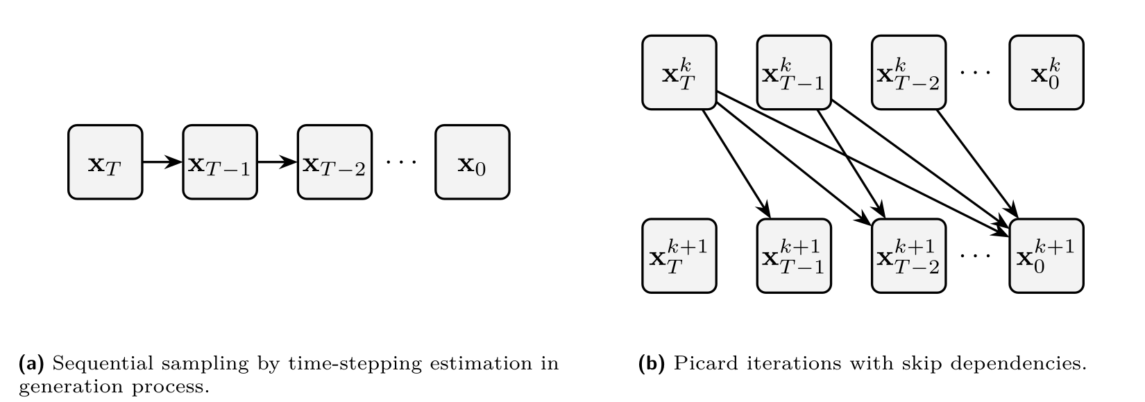
From Time-Stepping to Time-Parallel Solver
In the previous sections, we focused on the time–stepping approach, which estimates the trajectory by evolving from the prior time \(T\) toward an arbitrary \(t\in[0,T]\). Let \[{\mathbf{v}}_{{\bm{\phi}}^\times}({\mathbf{x}},t):={\mathbf{f}}({\mathbf{x}}, t) - \frac{1}{2}g^2(t) {\mathbf{s}}_{{\bm{\phi}}^\times}({\mathbf{x}},t)\] denote the empirical PF–ODE drift from a pre-trained diffusion model. The exact evolution from \(T\) to any intermediate time \(t\) is: \[\begin{equation} \label{eq:picard_T_to_t} \widetilde{\bm{\Psi}}_{T\to t}\big({\mathbf{x}}(T)\big) = {\mathbf{x}}(T) + \int_{T}^{t}{\mathbf{v}}_{{\bm{\phi}}^\times}\big({\mathbf{x}}(\tau),\tau\big)\mathop{}\!\mathrm{d}\tau, \quad {\mathbf{x}}(T)\sim p_{\mathrm{prior}}. \end{equation}\] Time–stepping schemes approximate this integral using discrete updates based on past timesteps.
In this section, we turn to the time–parallel approach, exemplified by ParaDiGMS, which builds on classical Picard iteration to enable parallel integration across time. The key idea behind ParaDiGMS is to trade computational resources for faster simulation.
Methodology of ParaDiGMS
From Trajectories to Picard Iteration as a Fixed-Point Update.
Fix the initial state of reverse-time sampling, \[{\mathbf{x}}_T\sim p_{\mathrm{prior}}.\] The integral expression in Equation \(\eqref{eq:picard_T_to_t}\) can be viewed as a map that takes an entire candidate trajectory and produces an updated one. Formally, given any path \(\{{\mathbf{y}}(\tau)\}_{\tau\in[0,T]}\), define \[(\mathcal{L}[{\mathbf{y}}(\cdot)])(t) = {\mathbf{x}}_T + \int_T^t {\mathbf{v}}_{{\bm{\phi}}^\times}\big({\mathbf{y}}(\tau),\tau\big)\mathop{}\!\mathrm{d}\tau, \qquad t\in[0,T].\] That is, \(\mathcal{L}\) keeps the initial state \({\mathbf{x}}_T\) fixed and updates the rest of the trajectory using the velocity evaluated along the candidate path.
A solution trajectory \({\mathbf{x}}^*(\cdot)\) of the empirical PF-ODE with \({\mathbf{x}}^*(T)={\mathbf{x}}_T\) is precisely a fixed point of this map: \[{\mathbf{x}}^*(t) = \mathcal{L}[{\mathbf{x}}^*(\cdot)](t) = {\mathbf{x}}_T + \int_T^t {\mathbf{v}}_{{\bm{\phi}}^\times}\big({\mathbf{x}}^*(\tau),\tau\big)\mathop{}\!\mathrm{d}\tau.\] Thus, instead of constructing the trajectory strictly one time step after another, we may search for an entire trajectory that is consistent with this integral equation.
Starting from an initial guess \({\mathbf{x}}^{(0)}(\cdot)\) satisfying \({\mathbf{x}}^{(0)}(T)={\mathbf{x}}_T\), for example the constant path \({\mathbf{x}}^{(0)}(t)\equiv{\mathbf{x}}_T\), Picard iteration repeatedly applies this map: \[\begin{align} \label{eq:picard_iter_T_to_t} {\mathbf{x}}^{(k+1)}(t) = \mathcal{L}[{\mathbf{x}}^{(k)}(\cdot)](t) = {\mathbf{x}}_T + \int_T^t {\mathbf{v}}_{{\bm{\phi}}^\times} \big({\mathbf{x}}^{(k)}(\tau),\tau\big)\mathop{}\!\mathrm{d}\tau, \end{align}\] with \(k=0,1,2,\ldots\). Each iteration evaluates the velocity along the previous trajectory and uses these evaluations to update the trajectory at all time points.
Discrete Picard on a \(T\) to \(0\) Grid.
To turn Equation \(\eqref{eq:picard_iter_T_to_t}\) into a practical algorithm, we place a uniform, decreasing grid on \([0,T]\) by choosing a step count \(M\), setting \(\Delta t := T/M\), and defining \[t_j := T - j \Delta t, \quad j=0,1,\ldots,M,\] so \(t_0=T\) and \(t_M=0\). Denote sampled iterates by \[{\mathbf{x}}^{(k)}_j := {\mathbf{x}}^{(k)}(t_j).\] Because the grid runs reversely in time, the integral from \(T\) to \(t_j\) has negative orientation. Approximating it by left endpoints on the partition \(\{[t_{i+1},t_i]\}_{i=0}^{j-1}\) gives \[\int_{T}^{t_j}{\mathbf{v}}_{{\bm{\phi}}^\times}({\mathbf{x}}^{(k)}(\tau), \tau) \mathop{}\!\mathrm{d}\tau \approx - \Delta t \sum_{i=0}^{j-1} {\mathbf{v}}_{{\bm{\phi}}^\times}\big({\mathbf{x}}^{(k)}_{i}, t_i\big),\] since each small integral over \([t_{i+1},t_i]\) equals \(- \int_{t_i}^{t_{i+1}} \cdot\mathop{}\!\mathrm{d}\tau\). Substituting this approximation into Equation \(\eqref{eq:picard_iter_T_to_t}\) yields the discrete Picard update \[\begin{equation} \label{eq:discrete_picard_decreasing} {\mathbf{x}}^{(k+1)}_j = {\mathbf{x}}_T - \Delta t \underbrace{ \sum_{i=0}^{j-1} {\mathbf{v}}_{{\bm{\phi}}^\times} \big({\mathbf{x}}^{(k)}_i,t_i\big) }_{\substack{\text{cumulative sum}\\\ text{of drifts}}}, \qquad j=1,\ldots,M. \end{equation}\] This scheme is simple and parallel-friendly: each drift evaluation \({\mathbf{v}}_{{\bm{\phi}}^\times} \big({\mathbf{x}}^{(k)}_i,t_i\big)\) depends only on the previous iterate at the same time node \(t_i\), so all \(i=0,\dots,j - 1\) evaluations can be computed independently across the grid. The integral is then recovered by a cumulative sum, performed either serially or via a parallel prefix-sum (scan/sliding windows).
Sliding Windows and Parallel Evaluation.
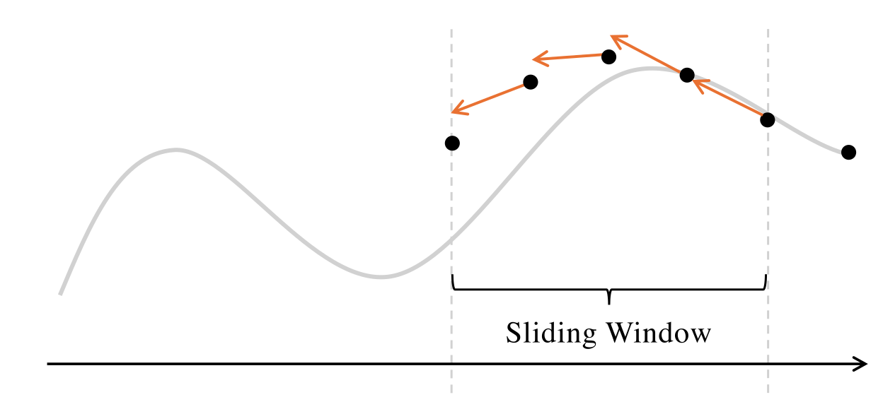
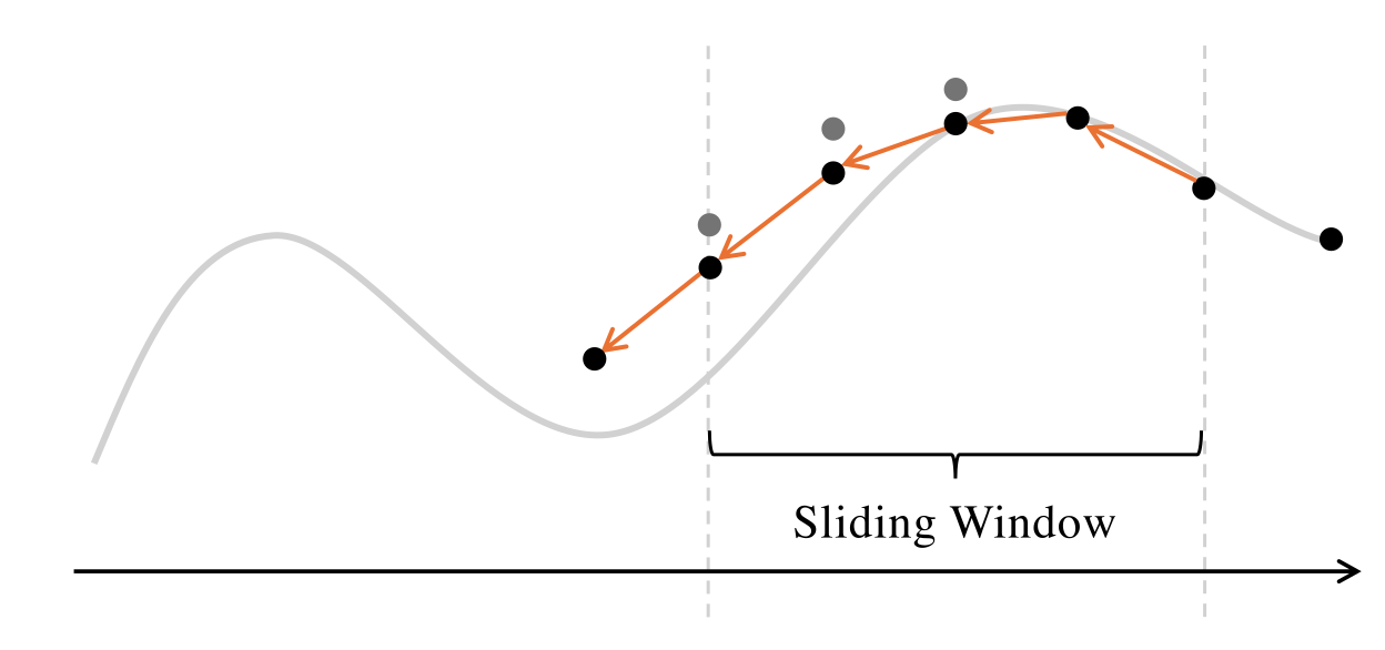
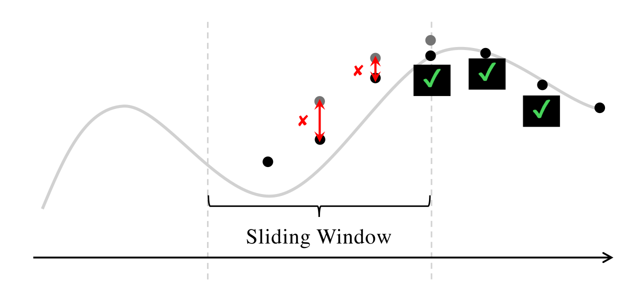
The discrete Picard update Equation \(\eqref{eq:discrete_picard_decreasing}\) expresses each \({\mathbf{x}}^{(k+1)}_j\) as the fixed initial value \({\mathbf{x}}_T\) minus a cumulative sum of drifts. To limit memory and exploit parallel hardware, it is convenient to apply the same idea locally on short, sliding blocks of indices.
Fix a window length \(p\) and a left index \(\ell\); the window then covers \(j=\ell,\ldots,\ell+p\) with \(t_\ell>t_{\ell+1}>\cdots>t_{\ell+p}\). During iteration \(k\):
Step 1. Parallel Drift Evaluation on the Window.
Compute, in parallel and using only the previous iterate, \[{\mathbf{v}}_{{\bm{\phi}}^\times} \big({\mathbf{x}}^{(k)}_{\ell+i}, t_{\ell+i}\big), \quad i=0,1,\ldots,p-1.\] These are the \(p\) local increments needed to advance from the left edge \(t_\ell\) across the window.
Step 2. Left–Anchored Cumulative Updates.
Form the windowed updates by anchoring at \(j=\ell\) and accumulating the drift across subintervals: \[\begin{equation} \label{eq:window_update} {\mathbf{x}}^{(k+1)}_{\ell+j+1} = {\mathbf{x}}^{(k)}_{\ell} - \Delta t \sum_{i=0}^{j} {\mathbf{v}}_{{\bm{\phi}}^\times} \big({\mathbf{x}}^{(k)}_{\ell+i}, t_{\ell+i}\big), \quad j=0,1,\ldots,p-1. \end{equation}\] This is the local, windowed counterpart of Equation \(\eqref{eq:discrete_picard_decreasing}\), with the current left-boundary value \({\mathbf{x}}^{(k)}_\ell\) serving as the anchor for the window. The minus sign reflects the decreasing time direction. The inner sum is a prefix sum over the windowed drifts, so all partial sums can be produced efficiently on parallel hardware.
Step 3. Progress Control and Window Advance.
Having formed the left–anchored cumulative updates on the current window (Step 2), we now decide how far to slide that window. We measure local convergence by the pointwise Picard change \[\mathtt{error}_j := \big\|{\mathbf{x}}^{(k+1)}_{\ell+j}-{\mathbf{x}}^{(k)}_{\ell+j}\big\|^2, \quad j=1,\ldots,p-1,\] and compare it against prescribed tolerances \(\mathtt{tol}_{\ell+j}\). That is, \(\mathtt{error}_j\) measures how much the iterate at node \(\ell+j\) changed during the last Picard update. If this number is small, it indicates local agreement between the two successive approximations and hence local convergence of the fixed-point iteration at that node. If it is large, that node has not settled yet and needs more Picard smoothing.
The stride is chosen as the first index in the window that fails this test (or the full window length \(p\) if none fail): \[\mathtt{stride} := \min\Big(\,\{\,j\ge 1:\ \mathtt{error}_j>\mathtt{tol}_{\ell+j}\,\}\ \cup\ \{p\}\Big).\] We then slide the window by setting \(\ell \leftarrow \ell+\mathtt{stride}\). In words: we accept all nodes from the left edge up to (but not including) the first one that has not converged; if all nodes have converged, we accept the entire window. We then slide the window by that many accepted nodes, \(\ell \leftarrow \ell+\mathtt{stride}\), and continue. This advances by at most the window length \(p\), never skipping any node that has not met its tolerance. If sliding would overrun the grid end \(M\), we truncate the window to \(p \leftarrow \min\{p,\,M-\ell\}\) and proceed.
When the window moves forward it uncovers new time nodes that have no values yet. To start Picard iteration there, we simply copy the value from the left boundary of the window and use it as an initial guess. This “constant extrapolation” is cheap and stable, and will be corrected by later updates. If desired, one can replace it by more accurate guesses, such as linear or polynomial extrapolations from past points.
This completes the procedure of ParaDiGMS. We summarize the algorithm in Algorithm (ParaDiGMS with Sliding Windows).
Algorithm: ParaDiGMS with Sliding Windows
Input: Drift \({\mathbf{v}}_{{\bm{\phi}}^\times}({\mathbf{x}},t)\); \(\{t_j\}_{j=0}^{M}\); window length \(p\); \(\{\mathtt{tol}_j\}_{j=1}^{M}\) Output: Approximate trajectory \(\{{\mathbf{x}}^{(k)}_j\}_{j=0}^{M}\) with \({\mathbf{x}}^{(k)}_M\) at \(t=0\)
\(k \gets 0\), \(\ell \gets 0\)
Sample \({\mathbf{x}}^{(0)}_0 \sim p_{\mathrm{prior}}\); set \({\mathbf{x}}^{(0)}_j \gets {\mathbf{x}}^{(0)}_0\) for \(j=1,\ldots,\min(p,M)\)
// constant extrapolation
while \(\ell < M\) do
\(J \gets \min(p, M-\ell)\) // current window length
Step 1: Parallel
For \(i=0,\ldots,J-1\): \(g_i \gets {\mathbf{v}}_{{\bm{\phi}}^\times} \big({\mathbf{x}}^{(k)}_{\ell+i},\, t_{\ell+i}\big)\)
// drifts from previous iterate (Picard freezing)
Compute prefix sums \(S_j \gets \sum_{i=0}^{j} g_i\) for \(j=0,\ldots,J-1\)
// scan over windowed drifts
Step 2: Cumulative Updates
For \(j=0,\ldots,J-1\): \(\displaystyle {\mathbf{x}}^{(k+1)}_{\ell+j+1} \gets {\mathbf{x}}^{(k)}_{\ell} - \Delta t\, S_j\)
// left-anchored update; cf. Equation \(\eqref{eq:window_update}\)
Step 3: Progress Control and Window Advance
For \(j=1,\ldots,J-1\): \(\mathtt{error}_j \gets \big\|{\mathbf{x}}^{(k+1)}_{\ell+j}-{\mathbf{x}}^{(k)}_{\ell+j}\big\|^2\)
// pointwise Picard change
\(\displaystyle \mathtt{stride} \gets \min \Big(\,\{\,j\in\{1,\ldots,J-1\}:~\mathtt{error}_j>\mathtt{tol}_{\ell+j}\,\}\ \cup\ \{J\}\Big)\)
Initialize New Nodes
For \(r=1,\ldots,\min\{\mathtt{stride},\,M-\ell-J\}\): \({\mathbf{x}}^{(k+1)}_{\ell+J+r} \gets {\mathbf{x}}^{(k+1)}_{\ell+J}\)
// constant extrapolation into newly exposed indices
\(\ell \gets \ell + \mathtt{stride}\);\(k \gets k+1\)
\(\{{\mathbf{x}}^{(k)}_j\}_{j=0}^{M}\)
Relation to Time-Stepping Solvers
Selection of Sliding Window Size.
To understand the role of the window size, first consider the smallest choice \(p=1\). In this case, there is no time parallelism, and the method reduces to its sequential base update. For the left-endpoint discretization in Equation \(\eqref{eq:window_update}\), this is simply a plain Euler step.
More generally, ParaDiGMS specifies how computations across different time points can be parallelized, while the numerical update used at each step can be chosen separately. For example, the Euler update can be replaced by DDIM or DPM-Solver, giving ParaDDIM or ParaDPMSolver. Increasing \(p\) then exposes more time points to parallel computation without changing the underlying time grid or the total number of steps \(M\). Picard iteration repeatedly corrects these states toward consistency with the chosen base solver, with convergence controlled by the prescribed local tolerances.
Compatibility with Higher–Order Solvers (e.g., DPM).
The Picard framework determines how states at different time points are updated and evaluated in parallel, while the numerical rule used to approximate each step can be chosen separately.
For example, instead of the left-endpoint rule in Equation \(\eqref{eq:window_update}\), we may use the trapezoidal rule: \[\begin{align*} {\mathbf{x}}^{(k+1)}_{\ell+j+1} = {\mathbf{x}}^{(k)}_{\ell} -\Delta t\Bigg[ \tfrac{1}{2} {\mathbf{v}}_{{\bm{\phi}}^\times} \big({\mathbf{x}}^{(k)}_{\ell},t_{\ell}\big) + \sum_{i=1}^{j} {\mathbf{v}}_{{\bm{\phi}}^\times} \big({\mathbf{x}}^{(k)}_{\ell+i},t_{\ell+i}\big) + \tfrac{1}{2} {\mathbf{v}}_{{\bm{\phi}}^\times} \big({\mathbf{x}}^{(k)}_{\ell+j+1},t_{\ell+j+1}\big) \Bigg], \end{align*}\] where \(j=0,\ldots,p-1\). For \(j=0\), this is the familiar one-step trapezoidal update using the two endpoint drifts. For larger \(j\), the same rule accumulates the trapezoidal contributions across the window. Since all drifts are evaluated using the previous Picard iterate, they can still be computed in parallel, while the interior contributions can be accumulated with a prefix sum.
More generally, ParaDiGMS can use an existing sequential sampler such as DDIM or DPM-Solver as its base discretization. In that case, the Picard update is constructed from the corresponding base-solver increment rather than from the trapezoidal formula above. The precise form depends on the chosen solver, since higher-order methods may use intermediate stages or previous model evaluations.
For a ParaDiGMS construction based on a given sequential solver, exact fixed-point convergence recovers the corresponding sequential discrete trajectory. With a finite stopping tolerance, the final result also contains a remaining fixed-point iteration error in addition to the discretization error of the base solver.
Closing Remarks
This chapter has confronted one of the most significant practical limitations of diffusion models: their slow, iterative sampling process. We have explored training-free approaches that accelerate generation by designing better numerical solvers for the empirical PF-ODE:
We began with DDIM, a first-order factored exponential-integrator update that retains the known diffusion schedule analytically while holding the neural prediction fixed.
We then studied DEIS, which extends this idea to higher-order multistep updates by reusing past model evaluations to extrapolate how the neural prediction changes.
Finally, we examined the DPM-Solver family, which introduces the log-SNR time coordinate and constructs higher-order updates from within-step model evaluations. DPM-Solver
++further develops single-step and multistep variants in the data-prediction formulation.
Together, these methods illustrate a common principle: exploit the analytically known diffusion structure and concentrate numerical approximation on the learned model prediction. They differ in the prediction and time parameterizations, and in whether higher-order information is obtained from within-step stages or previous-step history. ParaDiGMS provides a complementary direction by reorganizing computation across time through fixed-point iteration and parallel evaluation. Such solver developments can reduce the sampling cost from hundreds or thousands of model evaluations to only tens in many practical settings.
However, these training-free methods remain fundamentally iterative: they numerically approximate a continuous generative trajectory, even when parts of the computation can be parallelized. This raises a natural question: can we achieve high-quality generation in just one or a very few steps?
The final Part D of this monograph explores this question through training-based acceleration. In Chapter 10, we study distillation-based methods, where a fast student generator learns to reproduce the behavior of a slow pre-trained teacher. In Chapter 11, we turn to methods that directly learn few-step generators from scratch defined by an ODE flow.
This shift from designing a better numerical solver to directly learning a fast approximation of the generative solution map aims to combine the quality of diffusion models with the speed of one- or few-step generation.
To see the scaling, recall the oracle relation from Equation in Chapter 6 \[{\bm{\epsilon}}^*({\mathbf{x}}_t,t) = -\sigma_t\nabla_{{\mathbf{x}}}\log p_t({\mathbf{x}}_t),\] where \({\bm{\epsilon}}^*({\mathbf{x}}_t,t) = \mathbb{E}[{\bm{\epsilon}}|{\mathbf{x}}_t]\) is the oracle noise predictor, and the perturbation kernel is \({\mathbf{x}}_t|{\mathbf{x}}_0 \sim \mathcal{N}({\mathbf{x}}_t; \alpha_t{\mathbf{x}}_0,\sigma_t^2{\mathbf{I}})\). By the orthogonality property of conditional expectation in \(L^2\), \[\mathbb{E}\|{\bm{\epsilon}}\|_2^2 = \mathbb{E}\|{\bm{\epsilon}}^*\|_2^2 + \mathbb{E}\|{\bm{\epsilon}}-{\bm{\epsilon}}^*\|_2^2,\] and therefore \[\mathbb{E}\|{\bm{\epsilon}}^*\|_2^2 \le \mathbb{E}\|{\bm{\epsilon}}\|_2^2 = D,\] where \(D\) is the data dimension. Thus, the oracle noise predictor has uniformly bounded expected squared norm. In contrast, the oracle score \[{\mathbf{s}}^*({\mathbf{x}}_t,t) := \nabla_{{\mathbf{x}}}\log p_t({\mathbf{x}}_t)\] satisfies \[\mathbb{E}\|{\mathbf{s}}^*({\mathbf{x}}_t,t)\|_2^2 = \sigma_t^{-2}\, \mathbb{E}\|{\bm{\epsilon}}^*({\mathbf{x}}_t,t)\|_2^2 \le \frac{D}{\sigma_t^2}.\] Thus, direct score prediction can become increasingly poorly scaled as \(\sigma_t\) becomes small, since noise prediction is converted to the score through the factor \(1/\sigma_t\). This scaling can make direct score parameterization numerically less favorable near small noise levels.↩︎
In standard semilinear notation, \(b(t){\mathbf{N}}_{\bm{\phi}^\times}\) could be absorbed into a single nonlinear term. We keep the two factors separate because \(b(t)\) is known analytically from the noise schedule, whereas \({\mathbf{N}}_{\bm{\phi}^\times}\) requires a neural-network evaluation. This allows a solver to approximate the neural prediction inside the integral while retaining and analytically integrating the known schedule-dependent coefficient.↩︎
In the following sections, we switch between the SDE coefficients \((f(t),g(t))\) and the Gaussian perturbation kernel \({\mathbf{x}}_t | {\mathbf{x}}_0 \sim \mathcal{N} \bigl( {\mathbf{x}}_t; \alpha_t{\mathbf{x}}_0, \sigma_t^2{\mathbf{I}} \bigr)\). They are related by \[f(t) = \frac{\alpha_t'}{\alpha_t}, \qquad g^2(t) = \frac{\mathop{}\!\mathrm{d}}{\mathop{}\!\mathrm{d}t}\bigl(\sigma_t^2\bigr) - 2\frac{\alpha_t'}{\alpha_t}\sigma_t^2 = 2\sigma_t\sigma_t' - 2\frac{\alpha_t'}{\alpha_t}\sigma_t^2.\]↩︎
The update in Equation \(\eqref{eq:factored-ei-step}\) is not plain Euler in the original state and time variables. After an integrating-factor transformation of the state and, on intervals where the resulting time coordinate is monotone, a corresponding time reparameterization, it can be written as an ordinary explicit Euler step. We make this connection concrete for diffusion sampling in the DDIM section.↩︎
Throughout this chapter, \(\tilde{{\mathbf{x}}}_s\) denotes the state at time level \(s\) used to initialize the current solver step, typically obtained from a previous numerical step. The tilde distinguishes it from \({\mathbf{x}}_s\), which denotes an oracle sample from the exact diffusion distribution, either \({\mathbf{x}}_s \sim p_s\) or, conditioned on \({\mathbf{x}}_0\), \({\mathbf{x}}_s \sim p_s(\,\cdot \mid {\mathbf{x}}_0)\). Hence, \(\tilde{{\mathbf{x}}}_s\) need not be exactly distributed according to \(p_s\).↩︎
For the Markov forward process, \({\mathbf{x}}_0\to{\mathbf{x}}_t\to{\mathbf{x}}_s\) with \(t<s\), the conditional posterior \(p({\mathbf{x}}_t|{\mathbf{x}}_s,{\mathbf{x}}_0)\) satisfies \[p_t({\mathbf{x}}_t|{\mathbf{x}}_0) = \int p({\mathbf{x}}_t|{\mathbf{x}}_s,{\mathbf{x}}_0) \,p_s({\mathbf{x}}_s|{\mathbf{x}}_0) \mathop{}\!\mathrm{d}{\mathbf{x}}_s\] by the law of total probability.↩︎
“AB” refers to the Adams–Bashforth multistep principle, here applied within the exponential-integrator formulation (Hochbruck and Ostermann 2010).↩︎