Chapter 2: Variational Perspective: From VAEs to DDPMs

In this chapter we view diffusion models through a variational lens. We begin with the Variational Autoencoders (VAEs), which represent data with latent variables and are trained by maximizing a tractable lower bound on the log likelihood. In this setting a learned encoder maps observations to latents, and a learned decoder maps latents back to observations, closing the modeling loop.

Building on this pattern, hierarchical variants (Hierarchical VAEs) stack several latent layers to capture structure at multiple scales. With this setup, Denoising Diffusion Probabilistic Models (DDPM) conceptually follow the similar template: instead of jointly training both the encoder and decoder, the encoder is fixed as a forward noising process that gradually maps data to noise, and training learns a decoder that reverses this path in successive denoising steps. In this view, VAEs, hierarchical VAEs, and diffusion models all optimize a likelihood surrogate defined by a variational bound, providing a common foundation for the methods introduced here.

Variational Autoencoder

How can a neural network learn to generate realistic data? A natural starting point is the autoencoder, which consists of two networks: a deterministic encoder that compresses an input to a low-dimensional latent code, and a deterministic decoder that reconstructs the input from this code. Training minimizes the reconstruction error between the original input and its reconstruction. While this setup enables accurate reconstruction, the latent space is unstructured: randomly sampling latent codes usually produces meaningless outputs, limiting the model’s use for generation.

The Variational Autoencoder (VAE) (Kingma and Welling 2013) solves this by imposing a probabilistic structure on the latent space. This transforms the model from a simple reconstruction tool into a true generative model, capable of producing novel and realistic data.

Probabilistic Encoder and Decoder

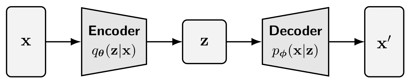
Construction of Decoder (Generator).

In VAEs, we distinguish between two types of variables: observed variables \({\mathbf{x}}\), which correspond to the data we see (e.g., an image), and latent variables \({\mathbf{z}}\), which capture the hidden factors of variation (e.g., object shape, color, or style). The model assumes that each observation \({\mathbf{x}}\) is generated from a latent variable sampled from a simple prior distribution, typically a standard Gaussian, \({\mathbf{z}}\sim p_{\text{prior}} := \mathcal{N}(\mathbf{0}, \mathbf{I})\).

To map \({\mathbf{z}}\) back to data space, we define a decoder (generator) distribution \(p_{\bm{\phi}}({\mathbf{x}}|{\mathbf{z}})\). In practice, this decoder is kept simple, often a factorized Gaussian (see Section 1.1.3) or similar distribution, so that learning focuses on extracting useful latent features rather than memorizing data. Intuitively, directly generating pixels one by one is extremely hard; instead, the latent variable provides a compact representation, from which decoding the exact pixel arrangement becomes much easier. New samples are drawn by first sampling \({\mathbf{z}}\sim p_{\text{prior}}\) and then decoding via \({\mathbf{x}}\sim p_{\bm{\phi}}({\mathbf{x}}|{\mathbf{z}})\).

The VAE thereby defines a latent-variable generative model through the marginal likelihood: \[p_{\bm{\phi}}({\mathbf{x}}) = \int p_{\bm{\phi}}({\mathbf{x}}|{\mathbf{z}}) p({\mathbf{z}}) \mathop{}\!\mathrm{d}{\mathbf{z}}.\] Ideally, the decoder parameters \(\bm{\phi}\) are learned by maximizing this marginal likelihood, as in maximum likelihood estimation (see Equation in Chapter 1). However, because the integral over \({\mathbf{z}}\) is intractable for expressive, non-linear decoders, direct MLE is computationally infeasible, motivating the variational approach used in VAEs.

Construction of Encoder (Inference Network).

To connect our intractable generator to real data, consider the reverse question: given an observation \({\mathbf{x}}\), what latent codes \({\mathbf{z}}\) could have produced it? By Bayes’ rule, the posterior distribution is \[p_{\bm{\phi}}({\mathbf{z}}|{\mathbf{x}}) \;=\; \frac{p_{\bm{\phi}}({\mathbf{x}}|{\mathbf{z}}) p({\mathbf{z}})}{p_{\bm{\phi}}({\mathbf{x}})}.\] The difficulty is that the denominator involves the marginal likelihood \(p_{\bm{\phi}}({\mathbf{x}})\), which requires integrating over all latent variables and is intractable for nonlinear decoders. Thus, exact inference of \({\mathbf{z}}\) from \({\mathbf{x}}\) is computationally prohibitive.

The “variational” step in VAEs addresses this by replacing the intractable posterior with a tractable approximation. We introduce an encoder (or inference network) \(q_{\bm{\theta}}({\mathbf{z}}|{\mathbf{x}})\), parameterized by a neural network, whose role is to serve as a learnable proxy: \[q_{\bm{\theta}}({\mathbf{z}}|{\mathbf{x}}) \;\approx\; p_{\bm{\phi}}({\mathbf{z}}|{\mathbf{x}}).\] In practice, the encoder maps each observed data point \({\mathbf{x}}\) to a distribution over latent codes, providing a feasible and trainable pathway from \({\mathbf{x}}\) back to \({\mathbf{z}}\) that enables learning.

Training via the Evidence Lower Bound (ELBO)

We now define a computable training objective. While we cannot directly optimize \(\log p_{\bm{\phi}}(\mathbf{x})\), we can maximize a lower bound on it—the Evidence Lower Bound (ELBO):

The ELBO objective naturally decomposes into two parts:

• Reconstruction: Encourages accurate recovery of \(\mathbf{x}\) from its latent code \(\mathbf{z}\). With Gaussian encoder and decoder assumptions, this term reduces exactly to the familiar reconstruction loss of an autoencoder (cf. Section 1.1.3). However, as in autoencoders, optimizing this term alone risks memorizing the training data, motivating an additional regularization.

• Latent KL: Encourages the encoder distribution \(q_{\bm{\theta}}(\mathbf{z}|\mathbf{x})\) to stay close to a simple Gaussian prior \(p_{\mathrm{prior}}(\mathbf{z})\). This regularization shapes the latent space into a smooth and continuous structure, enabling meaningful generation by ensuring that samples drawn from the prior can be reliably decoded.

This trade-off ensures both faithful reconstructions and coherent sampling.

Information-Theoretic View: ELBO as a Divergence Bound.

The ELBO objective has a natural information-theoretic interpretation. Recall that maximum likelihood training amounts to minimizing the KL divergence \[\mathcal{D}_{\mathrm{KL}}(p_{\text{data}}({\mathbf{x}}) \| p_{\bm{\phi}}({\mathbf{x}})),\] which measures how well the model distribution approximates the data distribution. Since this term is intractable in general, the variational framework introduces a joint comparison.

Specifically, consider two joint distributions:

• The generative joint, \(p_{\bm{\phi}}({\mathbf{x}}, {\mathbf{z}}) = p({\mathbf{z}}) p_{\bm{\phi}}({\mathbf{x}}|{\mathbf{z}})\), which describes how the model generates data;

• The inference joint, \(q_{\bm{\theta}}({\mathbf{x}}, {\mathbf{z}}) = p_{\text{data}}({\mathbf{x}}) q_{\bm{\theta}}({\mathbf{z}}|{\mathbf{x}})\), which couples real data with its inferred latent.

Comparing these distributions yields the inequality \[\begin{align} \label{eq:joint-bound} \mathcal{D}_{\mathrm{KL}}(p_{\text{data}}({\mathbf{x}}) \| p_{\bm{\phi}}({\mathbf{x}})) \leq \mathcal{D}_{\mathrm{KL}}(q_{\bm{\theta}}({\mathbf{x}},{\mathbf{z}}) \| p_{\bm{\phi}}({\mathbf{x}},{\mathbf{z}})), \end{align}\] sometimes referred to as the chain rule for KL divergence. Intuitively, comparing only marginals (\({\mathbf{x}}\)) can hide mismatches that are revealed when the full latent–data joint is considered.

Formally, one can expand the joint KL as \[\begin{align*} &\underbrace{\mathcal{D}_{\mathrm{KL}}(q_{\bm{\theta}}(\mathbf{x}, \mathbf{z}) \| p_{\bm{\phi}}(\mathbf{x}, \mathbf{z}))}_{\text{Total Error Bound}} \\=& \mathbb{E}_{q_{\bm{\theta}}(\mathbf{x}, \mathbf{z})} \left[ \log \frac{p_{\text{data}}(\mathbf{x}) q_{\bm{\theta}}(\mathbf{z}|\mathbf{x})}{p_{\bm{\phi}}(\mathbf{x}) p_{\bm{\phi}}(\mathbf{z}|\mathbf{x})} \right] \\=&\mathbb{E}_{p_{\text{data}}(\mathbf{x})} \left[ \log \frac{p_{\text{data}}(\mathbf{x})}{p_{\bm{\phi}}(\mathbf{x})} + \mathcal{D}_{\mathrm{KL}}\left( q_{\bm{\theta}}(\mathbf{z}|\mathbf{x}) \| p_{\bm{\phi}}(\mathbf{z}|\mathbf{x}) \right) \right] \\ \\=& \underbrace{\mathcal{D}_{\mathrm{KL}}(p_{\text{data}} \| p_{\bm{\phi}})}_{\text{True Modeling Error}} + \underbrace{\mathbb{E}_{p_{\text{data}}(\mathbf{x})} \big[ \mathcal{D}_{\mathrm{KL}}( q_{\bm{\theta}}(\mathbf{z}|\mathbf{x}) \| p_{\bm{\phi}}(\mathbf{z}|\mathbf{x}) ) \big]}_{\text{Inference Error}}, \end{align*}\] where the first term is the true modeling error and the second is the inference error, i.e., the gap between the approximate and true posteriors. The latter is always non-negative, which explains Equation \(\eqref{eq:joint-bound}\).

Finally, note that \[\log p_{\bm{\phi}}({\mathbf{x}}) - \mathcal{L}_{\text{ELBO}}(\bm{\theta},\bm{\phi};{\mathbf{x}}) = \mathcal{D}_{\mathrm{KL}} \left(q_{\bm{\theta}}({\mathbf{z}}|{\mathbf{x}})\|p_{\bm{\phi}}({\mathbf{z}}|{\mathbf{x}})\right).\] Thus the inference error is exactly the gap between the log-likelihood and the ELBO. Maximizing the ELBO therefore corresponds to directly reducing inference error, ensuring that training minimizes a meaningful part of the overall bound.

Gaussian VAE

A standard formulation of the VAE employs Gaussian distributions for both the encoder and decoder.

Encoder Part.

The encoder \(q_{\bm{\theta}}(\mathbf{z} | \mathbf{x})\) is typically modeled as a Gaussian distribution as: \[q_{\bm{\theta}}(\mathbf{z} | \mathbf{x}) := \mathcal{N}\left(\mathbf{z}; \bm{\mu}_{\bm{\theta}}(\mathbf{x}), \operatorname{diag}(\bm{\sigma}_{\bm{\theta}}^2(\mathbf{x}))\right),\] where \(\bm{\mu}_{\bm{\theta}} : \mathbb{R}^D \to \mathbb{R}^d\) and \(\bm{\sigma}_{\bm{\theta}} : \mathbb{R}^D \to \mathbb{R}_+^d\) are deterministic outputs of the encoder network.

Decoder Part.

The decoder is typically modeled as a Gaussian distribution with fixed variance: \[p_{\bm{\phi}}(\mathbf{x}|\mathbf{z}) := \mathcal{N}\bigl(\mathbf{x}; \bm{\mu}_{\bm{\phi}}(\mathbf{z}), \sigma^2 {\mathbf{I}}\bigr),\] where \(\bm{\mu}_{\bm{\phi}} : \mathbb{R}^d \to \mathbb{R}^D\) is a neural network, and \(\sigma > 0\) is a small constant controlling the variance.

Under this assumption, the reconstruction term in the ELBO simplifies as \[\mathbb{E}_{q_{\bm{\theta}}(\mathbf{z} | \mathbf{x})} \left[\log p_{\bm{\phi}}(\mathbf{x} | \mathbf{z})\right] = - \frac{1}{2\sigma^2} \mathbb{E}_{q_{\bm{\theta}}(\mathbf{z} | \mathbf{x})} \left[\|\mathbf{x} - \bm{\mu}_{\bm{\phi}}(\mathbf{z})\|^2\right] + C,\] where \(C\) is a constant independent of \(\bm{\theta}\) and \(\bm{\phi}\). The ELBO objective thus reduces to: \[\min_{\bm{\theta}, \bm{\phi}} \mathbb{E}_{q_{\bm{\theta}}(\mathbf{z} | \mathbf{x})} \left[ \frac{1}{2\sigma^2} \|\mathbf{x} - \bm{\mu}_{\bm{\phi}}(\mathbf{z})\|^2 \right] + \mathcal{D}_{\mathrm{KL}}\big(q_{\bm{\theta}}(\mathbf{z} | \mathbf{x}) \| p_{\mathrm{prior}}(\mathbf{z})\big),\] where the KL term admits a closed-form solution due to the Gaussian assumption. Training the VAE therefore reduces to minimizing a regularized reconstruction loss.

Drawbacks of Standard VAE

Despite the theoretical appeal of the VAE framework, it suffers from a critical drawback: it often produces blurry outputs¹.

Blurry Generations in VAEs.

To understand this phenomenon, consider a fixed Gaussian encoder \(q_{\text{enc}}(\mathbf{z}|\mathbf{x})\), and a decoder of the form \[p_{\text{dec}}(\mathbf{x}|\mathbf{z}) = \mathcal{N}(\mathbf{x}; \bm{\mu}({\mathbf{z}}), \sigma^2 {\mathbf{I}}),\] where \(\bm{\mu}({\mathbf{z}})\) denotes the decoder network. With an arbitrary encoder, optimizing the ELBO reduces (up to an additive constant) to minimizing the expected reconstruction error: \[\mathop{\mathrm{arg\,min}}_{\bm{\mu}} \mathbb{E}_{p_{\text{data}}(\mathbf{x})q_{\text{enc}}(\mathbf{z}|\mathbf{x})} \left[ \| \mathbf{x} - \bm{\mu}({\mathbf{z}}) \|^2 \right].\] This is a standard least squares problem in \(\bm{\mu}({\mathbf{z}})\), and its solution is given in closed form by the conditional mean: \[\bm{\mu}^*(\mathbf{z}) = \mathbb{E}_{q_{\text{enc}}(\mathbf{x}|\mathbf{z})}[\mathbf{x}],\] where \(q_{\text{enc}}(\mathbf{x}|\mathbf{z})\) is the encoder-induced posterior on inputs given latents, defined via Bayes’ rule: \[q_{\text{enc}}(\mathbf{x}|\mathbf{z}) = \frac{q_{\text{enc}}(\mathbf{z}|\mathbf{x})\, p_{\text{data}}(\mathbf{x})}{q_{\text{enc}}(\mathbf{z})}, \qquad q_{\text{enc}}(\mathbf{z}) := \int q_{\text{enc}}(\mathbf{z}|\mathbf{x})\, p_{\text{data}}(\mathbf{x})\, \mathop{}\!\mathrm{d}\mathbf{x}.\]

An equivalent form of the optimal generator via Bayes’ rule is: \[\bm{\mu}^*(\mathbf{z}) = \frac{\mathbb{E}_{p_{\text{data}}(\mathbf{x})}\!\left[q_{\text{enc}}(\mathbf{z}|\mathbf{x}) \cdot \mathbf{x}\right]} {q_{\text{enc}}(\mathbf{z})} = \frac{\mathbb{E}_{p_{\text{data}}(\mathbf{x})}\!\left[q_{\text{enc}}(\mathbf{z}|\mathbf{x}) \cdot \mathbf{x}\right]} {\mathbb{E}_{p_{\text{data}}(\mathbf{x})}\!\left[q_{\text{enc}}(\mathbf{z}|\mathbf{x})\right]}.\] Now suppose that two distinct inputs \(\mathbf{x} \neq \mathbf{x}'\) are mapped to overlapping regions in latent space, i.e., the supports of \(q_{\text{enc}}(\cdot|\mathbf{x})\) and \(q_{\text{enc}}(\cdot|\mathbf{x}')\) intersect. Then \(\bm{\mu}^*(\mathbf{z})\) averages over multiple, potentially unrelated inputs, which leads to blurry, non-distinct outputs. This averaging effect over conflicting modes is a fundamental reason for the characteristic blurriness in VAE-generated samples.

(Optional) From Standard VAE to Hierarchical VAEs

To model complex data, Hierarchical Variational Autoencoders (HVAEs) (Vahdat and Kautz 2020) enhance VAEs by introducing a hierarchy of latent variables. This deep, layered structure allows the model to capture data features at multiple levels of abstraction, significantly boosting expressive power and mirroring the compositional nature of real-world data.

HVAE’s Modeling.

Unlike standard VAEs that use a single latent code \(\mathbf{z}\), hierarchical VAEs (HVAEs) introduce multiple layers of latent variables arranged in a top-down hierarchy. Each latent layer conditions the one below it, forming a chain of conditional priors that captures structure at progressively finer levels of abstraction. This leads to the following top-down factorization of the joint distribution:

\[p_{\bm{\phi}}(\mathbf{x}, \mathbf{z}_{1:L}) = p_{\bm{\phi}}(\mathbf{x} | \mathbf{z}_1) \prod_{i=2}^{L} p_{\bm{\phi}}(\mathbf{z}_{i-1}|\mathbf{z}_i) p(\mathbf{z}_L).\] This structure defines the marginal data distribution, \[p_{\text{HVAE}}(\mathbf{x}) := \int p_{\bm{\phi}}(\mathbf{x}, \mathbf{z}_{1:L}) \mathop{}\!\mathrm{d}\mathbf{z}_{1:L}.\] Generation proceeds progressively: starting from the top latent variable \(\mathbf{z}_L\), each latent is decoded sequentially down to \(\mathbf{z}_1\), followed by generating the final observation \(\mathbf{x}\).

For encoding part, HVAEs utilize a structured, learnable variational encoder \(q_{\bm{\theta}}(\mathbf{z}_{1:L}|\mathbf{x})\) that mirrors the generative hierarchy. A common choice is a bottom-up Markov factorization: \[q_{\bm{\theta}}(\mathbf{z}_{1:L} | \mathbf{x}) = q_{\bm{\theta}}(\mathbf{z}_1 | \mathbf{x}) \prod_{i=2}^{L} q_{\bm{\theta}}(\mathbf{z}_i | \mathbf{z}_{i-1}).\]

HVAE’s ELBO.

Similar to Equation \(\eqref{eq:vae-elbo}\), ELBO is derived via Jensen’s inequality: \[\begin{align} \label{eq:hvae-elbo} \begin{aligned} \log p_{\text{HVAE}}(\mathbf{x}) &= \log \int p_{\bm{\phi}}(\mathbf{x}, \mathbf{z}_{1:L}) \mathop{}\!\mathrm{d}\mathbf{z}_{1:L} \\ &= \log \int \frac{p_{\bm{\phi}}(\mathbf{x}, \mathbf{z}_{1:L})}{q_{\bm{\theta}}(\mathbf{z}_{1:L}|\mathbf{x})} q_{\bm{\theta}}(\mathbf{z}_{1:L}|\mathbf{x}) \mathop{}\!\mathrm{d}\mathbf{z}_{1:L} \\ &= \log \mathbb{E}_{q_{\bm{\theta}}(\mathbf{z}_{1:L}|\mathbf{x})} \left[ \frac{p_{\bm{\phi}}(\mathbf{x}, \mathbf{z}_{1:L})}{q_{\bm{\theta}}(\mathbf{z}_{1:L}|\mathbf{x})} \right] \\ &\geq \mathbb{E}_{q_{\bm{\theta}}(\mathbf{z}_{1:L}|\mathbf{x})} \left[ \log \frac{p_{\bm{\phi}}(\mathbf{x}, \mathbf{z}_{1:L})}{q_{\bm{\theta}}(\mathbf{z}_{1:L}|\mathbf{x})} \right]\\ &=:\mathcal{L}_{\text{ELBO}}(\bm{\phi}). \end{aligned} \end{align}\] Substituting the factorized forms yields: \[\begin{align*} \mathcal{L}_{\text{ELBO}} = \mathbb{E}_{q_{\bm{\theta}}(\mathbf{z}_{1:L}|\mathbf{x})} \left[ \log \frac{ p(\mathbf{z}_L) \prod_{i=2}^{L} p_{\bm{\phi}}(\mathbf{z}_{i-1} | \mathbf{z}_i) p_{\bm{\phi}}(\mathbf{x} | \mathbf{z}_1) }{ q_{\bm{\theta}}(\mathbf{z}_1|\mathbf{x}) \prod_{i=2}^{L} q_{\bm{\theta}}(\mathbf{z}_i|\mathbf{z}_{i-1}) } \right]. \end{align*}\]

This hierarchical ELBO decomposes into interpretable terms, including a reconstruction term, adjacent-layer matching terms, and a top-level KL regularizer to the prior.

The leap from shallow to deep networks revolutionized machine learning, and a similar idea transformed generative models. HVAEs showed the power of using deep, stacked layers to build data. This concept of a layered hierarchy is a cornerstone of modern generative modeling, appearing again in score-based methods (Section (Multi-Noise Levels of Denoising Score Matching (NCSN)Multi-Noise Levels of Denoising Score Matching (NCSN)) in Chapter 3) and normalizing flows (Section (Flow-Based Models: Normalizing Flows and Neural ODEs) in Chapter 5). The core insight is simple yet powerful:

Why Deeper Networks in a Flat VAE are Not Enough.

There are two fundamental limitations of a standard flat VAE that are not resolved by simply making the encoder and decoder deeper.

The first limitation is the variational family. In a standard VAE, \[q_{\bm{\theta}}({\mathbf{z}}| {\mathbf{x}})=\mathcal N \big({\mathbf{z}};\,\bm{\mu}_{{\bm{\theta}}}({\mathbf{x}}), \operatorname{diag}(\sigma_\theta^2({\mathbf{x}}))\big),\] so for each fixed \({\mathbf{x}}\) the encoder posterior is a single Gaussian with diagonal covariance. Greater network depth improves the accuracy of \(\bm{\mu}_{{\bm{\theta}}}\) and \(\sigma_{\bm{\theta}}\) but does not expand the family; even a full covariance remains one unimodal ellipsoid. When \(p_{\bm{\phi}}({\mathbf{z}}| {\mathbf{x}})\) is multi-peaked, this family cannot match it, which loosens the ELBO and weakens inference. Addressing this requires a richer posterior class, not merely deeper networks.

Second, if the decoder is too expressive, the model may suffer from posterior collapse. To see why, let us recall that the objective of the VAE is \[\begin{align*} &\mathbb{E}_{p_{\text{data}}(\mathbf{x})}[\mathcal L_{\mathrm{ELBO}}({\mathbf{x}})]\\ &\quad\quad=\mathbb{E}_{p_{\text{data}}(\mathbf{x})q_{\bm{\theta}}({\mathbf{z}}|{\mathbf{x}})}[\log p_{\bm{\phi}}({\mathbf{x}}|{\mathbf{z}})] -\mathbb{E}_{p_{\text{data}}(\mathbf{x})}\big[\mathcal{D}_\mathrm{KL} \big(q_{\bm{\theta}}({\mathbf{z}}|{\mathbf{x}}) \| p({\mathbf{z}})\big)\big]\\ &\quad\quad=\mathbb{E}_{p_{\text{data}}(\mathbf{x})q_{\bm{\theta}}({\mathbf{z}}|{\mathbf{x}})}[\log p_{\bm{\phi}}({\mathbf{x}}|{\mathbf{z}})]-\mathcal I_q({\mathbf{x}};{\mathbf{z}}) - \mathcal{D}_\mathrm{KL}(q_{\bm{\theta}}({\mathbf{z}}) \| p({\mathbf{z}})), \end{align*}\] where \(\mathcal I_q({\mathbf{x}};{\mathbf{z}})\) is the mutual information defined by \[\mathcal I_q({\mathbf{x}};{\mathbf{z}}) =\mathbb{E}_{q({\mathbf{x}},{\mathbf{z}})} \Big[\log \tfrac{q_{\bm{\theta}}({\mathbf{z}}|{\mathbf{x}})}{q({\mathbf{z}})}\Big] =\mathbb{E}_{p_{\mathrm{data}}({\mathbf{x}})} \big[\mathcal{D}_\mathrm{KL}(q_{\bm{\theta}}({\mathbf{z}}|{\mathbf{x}}) \| q({\mathbf{z}}))\big],\] and the aggregated posterior is \(q_{\bm{\theta}}({\mathbf{z}})= \int p_{\mathrm{data}}({\mathbf{x}}) q_{\bm{\theta}}({\mathbf{z}}|{\mathbf{x}}) \mathop{}\!\mathrm{d}{\mathbf{x}}\).

If the decoder class can model the data well without using \({\mathbf{z}}\) (i.e., it contains some \(p_{\bm{\phi}}({\mathbf{x}}|{\mathbf{z}})=r({\mathbf{x}})\) close to \(p_{\mathrm{data}}\)), then a maximizer of the ELBO sets \(q_{\bm{\theta}}({\mathbf{z}}|{\mathbf{x}})=p({\mathbf{z}})\), so \(\mathcal I_q({\mathbf{x}};{\mathbf{z}})=0\) and \(q_{\bm{\theta}}({\mathbf{z}})=p({\mathbf{z}})\). This “ignore \({\mathbf{z}}\)” solution does not disappear by making the networks deeper: (1) the learned code becomes independent of \({\mathbf{x}}\) (so it carries no data-dependent structure useful for downstream tasks), and (2) conditioning or moving in \({\mathbf{z}}\) has no effect on generated samples, so controllable generation fails.

What Hierarchy Changes?

An HVAE introduces multiple latent levels, \[p_{\bm{\phi}}({\mathbf{x}},{\mathbf{z}}_{1:L})=p_{\bm{\phi}}({\mathbf{x}}|{\mathbf{z}}_1)\prod_{i=2}^L p_{\bm{\phi}}({\mathbf{z}}_{i-1}|{\mathbf{z}}_i) p({\mathbf{z}}_L),\] with ELBO \[\begin{align*} \mathcal L_{\mathrm{ELBO}}({\mathbf{x}}) &= \mathbb{E}_{q_{\bm{\theta}}({\mathbf{z}}_1|{\mathbf{x}})}[\log p_{\bm{\phi}}({\mathbf{x}}|{\mathbf{z}}_1)] \\ &\quad - \mathbb{E}_{q_{\bm{\theta}}({\mathbf{z}}_{1:2}|{\mathbf{x}})} \big[\log q_{\bm{\theta}}({\mathbf{z}}_1|{\mathbf{x}})-\log p_{\bm{\phi}}({\mathbf{z}}_1|{\mathbf{z}}_2)\big] \\ &\quad - \sum_{i=2}^{L-1} \mathbb{E}_{q_{\bm{\theta}}({\mathbf{z}}_{1:i+1}|{\mathbf{x}})} \big[\log q_{\bm{\theta}}({\mathbf{z}}_i|{\mathbf{z}}_{i-1})-\log p_{\bm{\phi}}({\mathbf{z}}_i|{\mathbf{z}}_{i+1})\big] \\ &\quad - \mathbb{E}_{q_{\bm{\theta}}({\mathbf{z}}_{L-1}|{\mathbf{x}})} \Big[\mathcal{D}_{\mathrm{KL}}(q_{\bm{\theta}}({\mathbf{z}}_L|{\mathbf{z}}_{L-1}) \| p({\mathbf{z}}_L))\Big]. \end{align*}\] Here, we denote \(\mathbb{E}_q := \mathbb{E}_{p_{\mathrm{data}}({\mathbf{x}}) q_{{\bm{\theta}}}({\mathbf{z}}_{1:L}|{\mathbf{x}})}\). Each latent level interacts only with its neighboring levels in the hierarchy: the encoder passes information upward through \(q_{\bm{\theta}}({\mathbf{z}}_i|{\mathbf{z}}_{i-1})\), while the decoder passes information downward through \(p_{\bm{\phi}}({\mathbf{z}}_{i-1}|{\mathbf{z}}_i)\). Accordingly, the ELBO decomposes into a reconstruction term, adjacent-layer matching terms, and a top-level KL regularizer to the prior. These properties stem from the hierarchical latent graph, not from simply deepening networks in a flat VAE.

What Will be Ahead?

While HVAEs extend the VAE framework with multiple latent layers for expressiveness, their training poses unique challenges. Because the encoder and decoder must be optimized jointly, learning becomes unstable: lower layers and the decoder can already reconstruct \({\mathbf{x}}\), leaving higher-level latents with little effective signal. Moreover, gradient information reaching deeper variables is often indirect and weak, making it difficult for them to contribute meaningfully. An additional difficulty lies in balancing model capacity, since overly expressive conditionals can dominate the reconstruction task and suppress the utility of higher latents.

Interestingly, the core idea of a deep, layered hierarchy finds a more powerful incarnation in variational diffusion models, a topic we explore in Section 1.2. Diffusion models inherit the progressive structure of HVAEs but elegantly sidestep their central weakness. By fixing the encoding process and focusing solely on learning the generative reversal, they unlock newfound stability and modeling flexibility, leading to a significant leap in the quality of generated outputs.

For notational simplicity, we deviate from the common VAE convention that uses \(q\) for the encoder and \(p\) for the generator. To avoid ambiguity, we denote distributions as \(p\) and will always specify their roles through appropriate subscripts or superscripts, clarifying them in context.

Variational Perspective: DDPM

Denoising Diffusion Probabilistic Models (DDPMs) (Sohl-Dickstein et al. 2015; Ho et al. 2020) represent a cornerstone of diffusion modeling. Conceptually, they operate within a variational framework, much like VAEs and HVAEs. However, DDPMs introduce a clever twist that tackles some of the challenges faced by their predecessors.

At their core, DDPMs involve two distinct stochastic processes:

• The Forward Pass (Fixed Encoder): This process gradually corrupts data by injecting Gaussian noise over multiple steps via a transition kernel \(p(\mathbf{x}_{i}|\mathbf{x}_{i-1})\). The data evolves into an isotropic Gaussian distribution, effectively becoming pure noise. This means the encoder is fixed and not learned.

• The Reverse Denoising Process (Learnable Decoder): Here, a neural network learns to reverse the noise corruption through a parameterized distribution \(p_{\bm{\phi}}(\mathbf{x}_{i-1}|\mathbf{x}_{i})\). Starting from pure noise, this process iteratively denoises to generate realistic samples. Crucially, each individual denoising step is a more manageable task than generating a complete sample from scratch, as VAEs often attempt to do.

By fixing the encoder and concentrating learning on the gradual generative trajectory, DDPMs achieve remarkable stability and expressive power.

In this section, we focus on DDPMs, postponing the broader discussion to Section (A Direct View Through Accumulated Perturbation KernelsA Direct View Through Accumulated Perturbation Kernels) in Chapter 4, where we present a more general and flexible framework.

Forward Process (Fixed Encoder)

In DDPMs, the forward process is a fixed, non-trainable operation that serves as an encoder. It progressively corrupts the original data by adding noise over multiple steps, eventually transforming it into a simple prior distribution \(p_{\text{prior}} := \mathcal{N}(\mathbf{0}, \mathbf{I})\). This transformation is depicted as the forward chain in Figure 1.3 or as illustrated in Figure 1.4.

Let us formalize this step-by-step degradation:

Fixed Gaussian Transitions.

Each step in the forward process is governed by a fixed Gaussian transition kernel²: \[p({\mathbf{x}}_i|{\mathbf{x}}_{i-1}) := \mathcal{N}({\mathbf{x}}_i; \sqrt{1 - \beta_i^2} {\mathbf{x}}_{i-1}, \beta_i^2 {\mathbf{I}}).\] Here, the process begins with \({\mathbf{x}}_{0}\), representing a sample drawn from the real data distribution \(p_{\text{data}}\). The sequence \(\{\beta_i\}_{i=1}^L\) denotes a pre-determined, monotonically increasing noise schedule, where each \(\beta_i \in (0, 1)\) controls the variance of the Gaussian noise injected at step \(i\). For convenience, we define \(\alpha_i := \sqrt{1 - \beta_i^2}\). This mathematical definition is precisely equivalent to the following intuitive iterative update: \[{\mathbf{x}}_i = \alpha_i {\mathbf{x}}_{i-1} + \beta_i \bm{\epsilon}_i,\] where \(\bm{\epsilon}_i \sim \mathcal{N}(\bm{0}, {\mathbf{I}})\) are independently and identically distributed. This means at each step \(i\), we scale down the previous state \({\mathbf{x}}_{i-1}\) by \(\alpha_i\) and add a controlled amount of Gaussian noise scaled by \(\beta_i\).

Perturbation Kernel and Prior Distribution.

By recursively applying the transition kernels, we obtain a closed-form expression for the distribution of noisy samples at step \(i\) given the original data \({\mathbf{x}}_0\): \[p_i({\mathbf{x}}_i|{\mathbf{x}}_0) = \mathcal{N}\left({\mathbf{x}}_i; \bar{\alpha}_i {\mathbf{x}}_0, (1 - \bar{\alpha}_i^2) {\mathbf{I}}\right),\] where \[\bar{\alpha}_i := \prod_{k=1}^i \sqrt{1-\beta_k^2} = \prod_{k=1}^i \alpha_k.\] This means we can sample \({\mathbf{x}}_i\) directly from \({\mathbf{x}}\) as \[\begin{align} \label{eq:ddpm-forward} {\mathbf{x}}_i = \bar{\alpha}_i {\mathbf{x}}_0 + \sqrt{1-\bar{\alpha}_i^2} \bm{\epsilon}, \quad \bm{\epsilon} \sim \mathcal{N}(\bm{0}, {\mathbf{I}}). \end{align}\] Let the noise schedule \(\{\beta_i\}_{i=1}^L\) be an increasing sequence, then the marginal distribution of the forward process converges as \[p_L(\mathbf{x}_L | {\mathbf{x}}_0) \longrightarrow \mathcal{N}(\mathbf{0}, \mathbf{I}) \quad \text{as } L \to \infty,\] which motivates the choice of the prior distribution as \[p_{\text{prior}} := \mathcal{N}(\mathbf{0}, \mathbf{I})\] with no reliance on data \({\mathbf{x}}_0\).

Reverse Denoising Process (Learnable Decoder)

At its core, the essence of DDPMs lies in their ability to reverse the controlled degradation imposed by the forward diffusion process. Starting from pure, unstructured noise, \(\mathbf{x}_L \sim p_{\text{prior}}\), the objective is to progressively denoise this randomness, step by step, until a coherent and meaningful data sample emerges. This reverse generation proceeds through a Markov chain, illustrated by Figure 1.5.

The fundamental challenge, and the central question guiding DDPM development, then becomes:

Rather than diving immediately into the mathematically intricate derivation of the Evidence Lower Bound (ELBO), as the original DDPM paper does (for which a detailed discussion awaits in Section 1.2.5), we will instead approach the training objective from a more intuitive perspective: by leveraging conditional probabilities to achieve a tractable formulation.

Overview: Modeling and Training Objective.

To enable the generative process, our goal is to approximate the unknown true reverse transition kernel, \(p(\mathbf{x}_{i-1}|\mathbf{x}_i)\). We achieve this by introducing a learnable parametric model, \(p_{\bm{\phi}}(\mathbf{x}_{i-1}|\mathbf{x}_i)\), and training it to minimize the expected KL divergence: \[\begin{align} \label{eq:marginal-kl-matching} \mathbb{E}_{p_i(\mathbf{x}_i)} \left[ \mathcal{D}_{\mathrm{KL}}\big(p(\mathbf{x}_{i-1}|\mathbf{x}_i) \| p_{\bm{\phi}}(\mathbf{x}_{i-1}|\mathbf{x}_i)\big) \right]. \end{align}\]

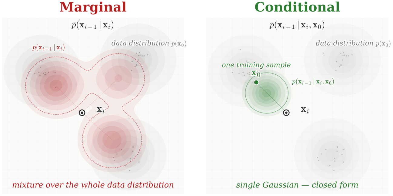
However, a direct computation of the target distribution \(p(\mathbf{x}_{i-1}|\mathbf{x}_i)\) is challenging. By Bayes’ theorem, we would need to evaluate: \[p(\mathbf{x}_{i-1}|\mathbf{x}_i) = p(\mathbf{x}_i|\mathbf{x}_{i-1}) \underbrace{\frac{p_{i-1}(\mathbf{x}_{i-1})}{p_i(\mathbf{x}_i)}}_{\text{intractable}}.\] The marginals \(p_i({\mathbf{x}}_i)\) and \(p_{i-1}({\mathbf{x}}_{i-1})\) are expectations over the unknown data distribution \(p_{\mathrm{data}}\), given by: \[p_i({\mathbf{x}}_i) = \int p_i({\mathbf{x}}_i | {\mathbf{x}}_0) p_{\mathrm{data}}({\mathbf{x}}_0) \mathrm{d}{\mathbf{x}}_0,\] and analogously for \(p_{i-1}({\mathbf{x}}_{i-1})\). Since \(p_{\mathrm{data}}\) is unknown, these integrals have no closed-form evaluation; at best they can be approximated from samples, so the exact densities are not available in practice.

Overcoming Intractability with Conditioning.

A central insight in DDPMs resolves this intractability: we condition the reverse transition on a clean data sample \(\mathbf{x}_0\). This subtle yet powerful step transforms the intractable kernel into one that is mathematically tractable: \[p(\mathbf{x}_{i-1}|\mathbf{x}_i, \mathbf{x}_0) = p(\mathbf{x}_i|\mathbf{x}_{i-1}) \frac{p(\mathbf{x}_{i-1}|\mathbf{x}_0)}{p_i(\mathbf{x}_i|\mathbf{x}_0)}.\] This tractability arises from two key properties of the forward process: its Markov property, meaning \(p(\mathbf{x}_i|\mathbf{x}_{i-1}, \mathbf{x}_0) = p(\mathbf{x}_i|\mathbf{x}_{i-1})\), and the Gaussian nature of all involved distributions. As a result, \(p(\mathbf{x}_{i-1}|\mathbf{x}_i, \mathbf{x}_0)\) itself is Gaussian and admits a closed-form expression (which we will see in Equation \(\eqref{eq:ddpm-reverse-mean}\)). We visualize it in Figure 1.6. Crucially, this elegant conditioning strategy allows us to derive a tractable objective that is functionally equivalent to the seemingly intractable marginal KL divergence in Equation \(\eqref{eq:marginal-kl-matching}\).

This alternative viewpoint: conditioning to obtain a tractable objective, forms the foundation of DDPMs and reveals a profound commonality with other influential diffusion models, as we will explore in Chapter 3 and Chapter 5.

It reveals a powerful equivalence: minimizing the KL divergence between marginal distributions is mathematically identical to minimizing the KL divergence between specific conditional distributions. This latter formulation is exceptionally useful because the crucial conditional distribution, \(p(\mathbf{x}_{i-1}|\mathbf{x}_i, \mathbf{x})\), possesses a convenient closed-form expression:

Later in Lemma in Chapter 4 (Reverse Conditional Transition Kernels), we present a more general formula that extends beyond the DDPM noising process described in Equation \(\eqref{eq:ddpm-forward}\).

Modeling of Reverse Transition Kernel \(p_{\bm{\phi}}(\mathbf{x}_{i-1}|\mathbf{x}_i)\)

Leveraging the gradient-level equivalence as in Theorem: Equivalence Between Marginal and Conditional KL Minimization and the Gaussian form of the reverse conditional \(p(\mathbf{x}_{i-1}|\mathbf{x}_i, \mathbf{x})\) as in Lemma: Reverse Conditional Transition Kernel, DDPM assumes that each reverse transition \(p_{\bm{\phi}}({\mathbf{x}}_{i-1}| {\mathbf{x}}_i)\) is Gaussian, parameterized as \[\begin{align} \label{eq:def-reverse} p_{\bm{\phi}}(\mathbf{x}_{i-1}|\mathbf{x}_i) := \mathcal{N}\big(\mathbf{x}_{i-1}; \bm{\mu}_{\bm{\phi}}(\mathbf{x}_i, i), \sigma^2(i) \mathbf{I}\big), \end{align}\] where \(\bm{\mu}_{\bm{\phi}}(\cdot, i) \colon \mathbb{R}^D \to \mathbb{R}^D\) is a learnable mean function, and \(\sigma^2(i) > 0\) is fixed as defined in Equation \(\eqref{eq:ddpm-reverse-mean}\).

We denote the KL divergence, averaged over time steps \(i\) and conditioned on data \({\mathbf{x}}_0 \sim p_{\text{data}}\), to match all layers of distributions as: \[\begin{align} \label{eq:ddpm-diffusion} \mathcal{L}_{\text{diffusion}}({\mathbf{x}}_0;\bm{\phi}) := \sum_{i=2}^L \mathbb{E}_{p_i({\mathbf{x}}_i|{\mathbf{x}}_0)}\left[\mathcal{D}_{\text{KL}}\big(p({\mathbf{x}}_{i-1}|{\mathbf{x}}_i, {\mathbf{x}}_0) \Vert p_{\bm{\phi}}({\mathbf{x}}_{i-1}|{\mathbf{x}}_i)\big)\right]. \end{align}\] Thanks to the Gaussian forms of both distributions and the parameterization defined in Equation \(\eqref{eq:def-reverse}\), the objective admits a closed-form expression and can be simplified as: \[\begin{align} \label{eq:ddpm-diffusion-simp} \mathcal{L}_{\text{diffusion}}({\mathbf{x}}_0;\bm{\phi}) = \sum_{i=2}^L \frac{1}{2\sigma^2(i)} \mathbb{E}_{p_i({\mathbf{x}}_i|{\mathbf{x}}_0)}\left\| \bm{\mu}_{\bm{\phi}}({\mathbf{x}}_i, i) - \bm{\mu}({\mathbf{x}}_i, {\mathbf{x}}_0, i) \right\|_2^2 + C, \end{align}\] where \(C\) is a constant independent of \(\bm{\phi}\). Averaging over the data distribution and omitting the constant \(C\) (which does not affect the optimization), the final DDPM training objective is \[\begin{align} \begin{aligned} \label{eq:ddpm-mean-loss} \mathcal{L}_{\text{DDPM}}(\bm{\phi}) := \sum_{i=2}^L \frac{1}{2\sigma^2(i)} \mathbb{E}_{{\mathbf{x}}_0} \mathbb{E}_{p_i({\mathbf{x}}_i|{\mathbf{x}}_0)} \left[ \left\| \bm{\mu}_{\bm{\phi}}(\mathbf{x}_i, i) - \bm{\mu}(\mathbf{x}_i, {\mathbf{x}}_0, i) \right\|_2^2 \right], \end{aligned} \end{align}\] where \({\mathbf{x}}_0\sim p_{\mathrm{data}}\).

We remark that the forward perturbation kernel \(p_i({\mathbf{x}}_i | {\mathbf{x}}_0)\) plays an important computational role in the training objective. It gives the distribution of the noisy state \({\mathbf{x}}_i\) obtained from a clean sample \({\mathbf{x}}_0\) after \(i\) forward steps. Because each forward transition is linear and Gaussian, their composition also has a closed-form Gaussian distribution; see the discussion around Equation \(\eqref{eq:ddpm-forward}\). Consequently, after selecting a time step \(i\), we can sample \({\mathbf{x}}_i \sim p_i({\mathbf{x}}_i | {\mathbf{x}}_0)\) directly from \({\mathbf{x}}_0\), without first generating the intermediate states \({\mathbf{x}}_1,\ldots,{\mathbf{x}}_{i-1}\). Thus, each loss term can be estimated using only a clean sample, a selected time step, and a directly corrupted sample, making stochastic training computationally efficient.

Practical Choices of Predictions and Loss

\({\bm{\epsilon}}\)-Prediction.

In typical DDPM implementations, training is not conducted directly using the original loss based on the mean prediction parameterization from Equation \(\eqref{eq:ddpm-mean-loss}\). Instead, an equivalent reparameterization, known as the \({\bm{\epsilon}}\)-prediction (noise prediction) formulation, is commonly adopted.

Recall that in the DDPM forward process, a noisy sample \({\mathbf{x}}_i \sim p({\mathbf{x}}_i |{\mathbf{x}}_0)\) at noise level \(i\) is generated by \[\begin{equation} \label{eq:ddpm-perturbation} {\mathbf{x}}_i = \bar{\alpha}_i {\mathbf{x}}_0 + \sqrt{1 - \bar{\alpha}_i^2} \boldsymbol{\epsilon}, \quad {\mathbf{x}}_0 \sim p_{\text{data}}, \quad \boldsymbol{\epsilon} \sim \mathcal{N}(\mathbf{0}, \mathbf{I}). \end{equation}\] Using this expression, the reverse mean \(\bm{\mu}({\mathbf{x}}_i, {\mathbf{x}}_0, i)\) from Equation \(\eqref{eq:ddpm-reverse-mean}\) can be rewritten as: \[\bm{\mu}({\mathbf{x}}_i, {\mathbf{x}}_0, i) = \frac{1}{\alpha_i} \left( {\mathbf{x}}_i - \frac{1 - \alpha_i^2}{\sqrt{1 - \bar{\alpha}_i^2}} \boldsymbol{\epsilon} \right).\]

This motivates a parameterization of the model mean \(\bm{\mu}_{\bm{\phi}}\) using a neural network \(\boldsymbol{\epsilon}_{\bm{\phi}}({\mathbf{x}}_i, i)\) that directly predicts the noise: \[\bm{\mu}_{\bm{\phi}}({\mathbf{x}}_i, i) = \frac{1}{\alpha_i} \left( {\mathbf{x}}_i - \frac{1 - \alpha_i^2}{\sqrt{1 - \bar{\alpha}_i^2}} \underbrace{\boldsymbol{\epsilon}_{\bm{\phi}}({\mathbf{x}}_i, i)}_{{\bm{\epsilon}}\text{-prediction}} \right).\] Substituting this into the original loss leads to a squared \(\ell_2\) error between predicted and true noise: \[\left\| \bm{\mu}_{\bm{\phi}}({\mathbf{x}}_i, i) - \bm{\mu}({\mathbf{x}}_i, {\mathbf{x}}_0, i) \right\|_2^2 \propto \left\| \boldsymbol{\epsilon}_{\bm{\phi}}({\mathbf{x}}_i, i) - \boldsymbol{\epsilon} \right\|_2^2,\] up to a weighting factor depending on \(i\). Intuitively, the model acts as a “noise detective”, estimating the random noise added at each step of the forward process. Subtracting this estimate from the corrupted sample moves it closer to the clean original, and repeating this step-by-step reconstructs the data from pure noise.

Simplified Loss with \({\bm{\epsilon}}\)-Prediction.

In practice, this expression is further simplified by omitting the weighting term, yielding the widely used DDPM training loss: \[\begin{equation} \label{eq:ddpm-simple-loss} \mathcal{L}_{\text{simple}}(\bm{\phi}) := \mathbb{E}_{i} \mathbb{E}_{{\mathbf{x}}\sim p_{\text{data}}({\mathbf{x}})} \mathbb{E}_{\boldsymbol{\epsilon} \sim \mathcal{N}(\mathbf{0}, \mathbf{I})} \left[ \left\| \boldsymbol{\epsilon}_{\bm{\phi}}({\mathbf{x}}_i, i) - \boldsymbol{\epsilon} \right\|_2^2 \right], \end{equation}\] where \({\mathbf{x}}_i = \bar{\alpha}_i {\mathbf{x}}_0 + \sqrt{1 - \bar{\alpha}_i^2} \boldsymbol{\epsilon}\) with \({\mathbf{x}}_0 \sim p_{\text{data}}\). Since the target noise has unit variance at every timestep \(t\), the \(\ell_2\) loss in Equation \(\eqref{eq:ddpm-simple-loss}\) maintains a consistent scale across all \(t\). This prevents vanishing or exploding targets and eliminates the need for explicit loss weighting.

Importantly, both \(\mathcal{L}_{\text{DDPM}}\) and \(\mathcal{L}_{\text{simple}}\) share the same optimal solution \(\boldsymbol{\epsilon}^*\), this is because Equation \(\eqref{eq:ddpm-simple-loss}\) essentially reduces to a least-squares problem (as shown similarly in Proposition in Chapter 4 (Minimizer of DSM) or Proposition in Chapter 6 (Equivalence of Parametrizations))³: \[\boldsymbol{\epsilon}^*({\mathbf{x}}_i, i) = \mathbb{E}\left[ \boldsymbol{\epsilon}|{\mathbf{x}}_i \right], \quad {\mathbf{x}}_i \sim p_i.\] Intuitively, the \({\bm{\epsilon}}\)-prediction network \(\boldsymbol{\epsilon}_{\bm{\phi}}({\mathbf{x}}_i, i)\) estimates the noise added by the forward process to produce \({\mathbf{x}}_i\). At optimality, this estimate coincides with the conditional expectation of the true noise, even though \({\mathbf{x}}_i\) does not uniquely determine the original clean sample.

Another Equivalent Parametrization: \({\mathbf{x}}\)-Prediction.

Equation \(\eqref{eq:ddpm-reverse-mean}\) motivates an alternative yet equivalent parameterization, known as \({\mathbf{x}}\)-prediction (clean prediction), in which a neural network \({\mathbf{x}}_{\bm{\phi}}({\mathbf{x}}_i, i)\) is trained to predict a clean (denoised) sample from a given noisy input \({\mathbf{x}}_i \sim p_i({\mathbf{x}}_i)\) at noise level \(i\). Replacing the ground-truth clean sample \({\mathbf{x}}_0\) in the reverse mean expression with \({\mathbf{x}}_{\bm{\phi}}({\mathbf{x}}_i, i)\) leads to the following model: \[\begin{align*} \bm{\mu}_{\bm{\phi}}({\mathbf{x}}_i, i) = \frac{\bar{\alpha}_{i-1} \beta_i^2}{1 - \bar{\alpha}_i^2} {\mathbf{x}}_{\bm{\phi}}({\mathbf{x}}_i, i) + \frac{(1 - \bar{\alpha}_{i-1}^2)\alpha_i}{1 - \bar{\alpha}_i^2} {\mathbf{x}}_i. \end{align*}\] Analogous to the \({\bm{\epsilon}}\)-prediction formulation, the training objective can be expressed as \[\left\| \bm{\mu}_{\bm{\phi}}({\mathbf{x}}_i, i) - \bm{\mu}({\mathbf{x}}_i, {\mathbf{x}}_0, i) \right\|_2^2 \propto \left\| {\mathbf{x}}_{\bm{\phi}}({\mathbf{x}}_i, i) - {\mathbf{x}}_0 \right\|_2^2, \quad {\mathbf{x}}_0 \sim p_{\text{data}},\] where the model is trained to predict the original data sample \({\mathbf{x}}_0\) from its noisy version \({\mathbf{x}}_i\). This equivalence reduces the mean-matching loss in Equation \(\eqref{eq:ddpm-mean-loss}\) to \[\mathbb{E}_{i} \mathbb{E}_{{\mathbf{x}}_0 \sim p_{\text{data}}} \mathbb{E}_{\boldsymbol{\epsilon} \sim \mathcal{N}(\mathbf{0}, \mathbf{I})} \left[\omega_i \left\| {\mathbf{x}}_{\bm{\phi}}({\mathbf{x}}_i, i) - {\mathbf{x}}_0 \right\|_2^2 \right],\] for some weighting function \(\omega_i\). Since this is a least-squares problem, the optimal solution is given by (see Proposition in Chapter 4 (Minimizer of DSM) or Proposition in Chapter 6 (Equivalence of Parametrizations)) \[\begin{align} \label{eq:ddpm-clean-minimizer} {\mathbf{x}}^*({\mathbf{x}}_i, i) = \mathbb{E}\left[ {\mathbf{x}}_0|{\mathbf{x}}_i \right], \quad {\mathbf{x}}_i \sim p_i, \end{align}\] that is, the model should predict the expected clean data given a noisy observation \({\mathbf{x}}_i\) at timestep \(i\).

The \({\mathbf{x}}\)-prediction and \({\bm{\epsilon}}\)-prediction parameterizations are mathematically equivalent and connected via the forward process: \[\begin{equation} \label{eq:ddpm-clean-noise} {\mathbf{x}}_i = \bar{\alpha}_i {\mathbf{x}}_{\bm{\phi}}({\mathbf{x}}_i, i) + \sqrt{1 - \bar{\alpha}_i^2} \boldsymbol{\epsilon}_{\bm{\phi}}({\mathbf{x}}_i, i). \end{equation}\] That is, one may either predict the clean sample \({\mathbf{x}}_{\bm{\phi}}({\mathbf{x}}_i, i)\) or the noise \(\boldsymbol{\epsilon}_{\bm{\phi}}({\mathbf{x}}_i, i)\), such that their combination reproduces \({\mathbf{x}}_i\) under the forward noising process.

DDPM’s ELBO

With the reverse transitions defined as in Equation \(\eqref{eq:def-reverse}\), this leads to the definition of the joint generative distribution in DDPM as: \[p_{\bm{\phi}}({\mathbf{x}}_0, {\mathbf{x}}_{1:L}) := p_{\bm{\phi}}({\mathbf{x}}_0|{\mathbf{x}}_1) p_{\bm{\phi}}({\mathbf{x}}_1|{\mathbf{x}}_2)\cdots p_{\bm{\phi}}({\mathbf{x}}_{L-1}|{\mathbf{x}}_L) p_{\text{prior}}({\mathbf{x}}_L),\] and the marginal generative model for data is given by: \[\begin{align*} p_{\bm{\phi}}({\mathbf{x}}_0) := \int p_{\bm{\phi}}({\mathbf{x}}_0, {\mathbf{x}}_{1:L}) \mathop{}\!\mathrm{d}{\mathbf{x}}_{1:L}. \end{align*}\]

Indeed, DDPM training via Equation \(\eqref{eq:ddpm-diffusion}\) can be rigorously grounded in maximum likelihood estimation (Equation in Chapter 1). Specifically, its objective forms an ELBO, similar to those in VAEs and HVAEs from Section 1.1, which serves as a lower bound on the log-density:

The ELBO \(\mathcal{L}_{\text{ELBO}}\) consists of three terms:

• \(\mathcal{L}_{\text{prior}}\) can be made negligible by choosing the noise schedule \(\{\beta_i\}\) such that \(p(\cdot|{\mathbf{x}}_0) \approx p_{\text{prior}}(\cdot)\).

• For \(\mathcal{L}_{\text{recon.}}\), this can be approximated and optimized using a Monte Carlo estimate; see (Ho et al. 2020; Kingma et al. 2021) for practical implementations.

• \(\mathcal{L}_{\text{diffusion}}\) (cf. Equation \(\eqref{eq:ddpm-diffusion}\)) matches the reverse conditionals \(p_{\bm{\phi}}(\mathbf{x}_{i-1}|\mathbf{x}_i)\) to \(p(\mathbf{x}_{i-1}|\mathbf{x}_i)\) at all steps \(i\).

The ELBO objective \(\mathcal{L}_{\text{ELBO}}\) can also be interpreted through the lens of the Data Processing Inequality with latents \({\mathbf{z}}= {\mathbf{x}}_{1:L}\), as illustrated in Equation \(\eqref{eq:joint-bound}\): \[\begin{align*} \mathcal{D}_{\mathrm{KL}}(p_{\mathrm{data}}({\mathbf{x}}_0) \| p_{\bm{\phi}}({\mathbf{x}}_0)) \leq \mathcal{D}_{\mathrm{KL}}\left(p({\mathbf{x}}_0, {\mathbf{x}}_{1:L}) \| p_{\bm{\phi}}({\mathbf{x}}_0, {\mathbf{x}}_{1:L})\right), \end{align*}\] where \(p({\mathbf{x}}_0, {\mathbf{x}}_{1:L}) := p_{\mathrm{data}}({\mathbf{x}}_0) p({\mathbf{x}}_1|{\mathbf{x}}_0) p({\mathbf{x}}_2|{\mathbf{x}}_1) \cdots p({\mathbf{x}}_L|{\mathbf{x}}_{L-1})\) denotes the joint distribution along the forward process.

Sampling

After training the \({\bm{\epsilon}}\)-prediction model, \(\bm{\epsilon}_{\bm{\phi}^\times}({\mathbf{x}}_i, i)\)⁴, sampling is performed sequentially as illustrated in Figure 1.5, using the parametrized transition \(p_{\bm{\phi}^\times}({\mathbf{x}}_{i-1} | {\mathbf{x}}_i)\) instead.

More specifically, starting from a random seed \({\mathbf{x}}_L \sim p_{\text{prior}} = \mathcal{N}(\bm{0},{\mathbf{I}})\), we recursively sample from \(p_{\bm{\phi}^\times}({\mathbf{x}}_{i-1} | {\mathbf{x}}_i)\) following the update rule below for \(i = L, L-1, \dots, 1\): \[\begin{align} \label{eq:ddpm-sampling} {\mathbf{x}}_{i-1} \leftarrow \underbrace{\frac{1}{\alpha_i}\left( {\mathbf{x}}_i - \frac{1-\alpha_i^2}{\sqrt{1-\bar{\alpha}_i^2}} \bm{\epsilon}_{\bm{\phi}^\times}({\mathbf{x}}_i, i)\right)}_{\bm{\mu}_{\bm{\phi}^\times}({\mathbf{x}}_i, i)} +\sigma(i) \bm{\epsilon}_i,\quad \bm{\epsilon}_i\sim \mathcal{N}(\bm{0},{\mathbf{I}}). \end{align}\] This “denoising” process continues until \({\mathbf{x}}_0\) is obtained as the final clean generated sample.

Another Interpretation of DDPM Sampling.

A useful way to interpret DDPM sampling is to rewrite the update rule so that the noise-level structure becomes explicit. Recall from Equation \(\eqref{eq:ddpm-clean-noise}\) that the predicted noise can be expressed in terms of the current sample \({\mathbf{x}}_i\) and the predicted clean sample \({\mathbf{x}}_{\bm{\phi}^\times}({\mathbf{x}}_i,i)\): \[\boldsymbol{\epsilon}_{\bm{\phi}^\times}({\mathbf{x}}_i,i) = \frac{{\mathbf{x}}_i - \bar{\alpha}_i\,{\mathbf{x}}_{\bm{\phi}^\times}({\mathbf{x}}_i,i)} {\sqrt{1-\bar{\alpha}_i^2}}.\] Substituting this into the DDPM sampling rule (Equation \(\eqref{eq:ddpm-sampling}\)) and rearranging, we obtain \[\begin{equation} \label{eq:ddpm-renoise} {\mathbf{x}}_{i-1} \;\leftarrow\; \bar{\alpha}_{i-1}\,{\mathbf{x}}_{\bm{\phi}^\times}({\mathbf{x}}_i,i) \;+\; \underbrace{ \sqrt{1-\bar{\alpha}_{i-1}^2 - \tilde{\beta}_i^2}\; \boldsymbol{\epsilon}_{\bm{\phi}^\times}({\mathbf{x}}_i,i) \;+\; \tilde{\beta}_i\,\boldsymbol{\epsilon}_i }_{\text{combined std.\ }=\;\sqrt{1-\bar{\alpha}_{i-1}^2}}, \end{equation}\] where \(\tilde{\beta}_i^2 = \frac{(1-\bar{\alpha}_{i-1}^2)(1-\alpha_i^2)}{1-\bar{\alpha}_i^2}\) is the DDPM posterior variance⁵. Moreover, the residual coefficients satisfy \[\bigl(1-\bar{\alpha}_{i-1}^2-\tilde{\beta}_i^2\bigr)+\tilde{\beta}_i^2 = 1-\bar{\alpha}_{i-1}^2,\] so the update has the same noise-level structure as the forward marginal at level \(i-1\). This returns to the first operational sampling template introduced in Equation in A First Operational View of Diffusion Model Training and Sampling predict the clean part and rewrite the sample at a lower noise level. DDPM carries out this rewrite stochastically, combining the noise direction estimated from \({\mathbf{x}}_i\) with a fresh Gaussian noise sample. A deterministic sampler follows the same basic idea, but removes the fresh randomness and adjusts the remaining noise coefficient accordingly. We will revisit this construction when studying diffusion samplers more systematically in Section (DDIMDDIM) in Chapter 9.

Compare Equation \(\eqref{eq:ddpm-renoise}\) with the forward marginal \({\mathbf{x}}_{i-1} = \bar{\alpha}_{i-1}\,{\mathbf{x}}_0 + \sqrt{1-\bar{\alpha}_{i-1}^2}\,\bar{\boldsymbol{\epsilon}}\). The structure is identical: signal coefficient \(\bar{\alpha}_{i-1}\) and noise standard deviation \(\sqrt{1-\bar{\alpha}_{i-1}^2}\), except that the unknown \({\mathbf{x}}_0\) is replaced by the network prediction \({\mathbf{x}}_{\bm{\phi}^\times}({\mathbf{x}}_i,i)\). In other words, each DDPM step predicts the clean data and then re-noises it to exactly noise level \(i{-}1\). One can therefore view DDPM sampling as iterating two operations:

1. Denoise. Estimate the clean data \({\mathbf{x}}_{\bm{\phi}^\times}({\mathbf{x}}_i, i)\) from the current noisy input \({\mathbf{x}}_i\).

2. Re-noise. Add back noise at the reduced level \(i{-}1\) via Equation \(\eqref{eq:ddpm-renoise}\), producing a sample \({\mathbf{x}}_{i-1}\) whose noise level matches the forward process at step \(i{-}1\).

However, even if \({\mathbf{x}}_{\bm{\phi}^\times}\) is trained as the optimal denoiser (i.e., the conditional expectation minimizer; see Equation \(\eqref{eq:ddpm-clean-minimizer}\)), it can only predict the average clean sample given \({\mathbf{x}}_i\). This limitation leads to blurry predictions, particularly at high noise levels, where recovering detailed structure from severely corrupted inputs becomes difficult. From this viewpoint, diffusion sampling moves from high to low noise and progressively refines an estimate of the clean signal. Early steps set the global structure, later steps add fine detail, and the sample becomes more realistic as the noise is removed.

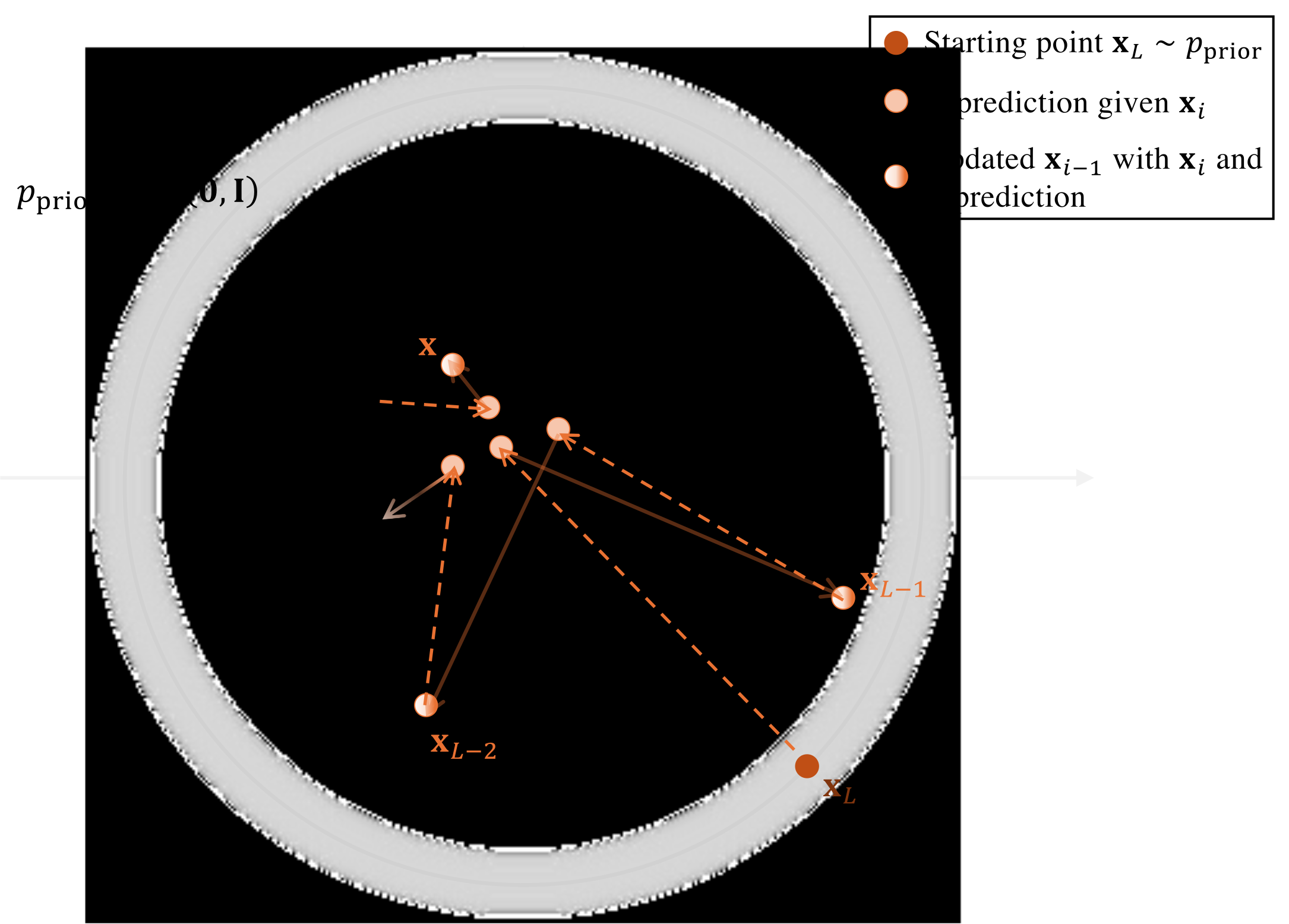
Slow Sampling Speed of DDPM.

Sampling in DDPMs (i.e., diffusion models) is inherently slow. In the original formulation and implementation, generating a sample typically requires around \(1{,}000\) denoising steps. This is because sampling proceeds through a long sequence of small refinements: at each step, the model updates the current noisy sample slightly toward a cleaner one, and the next update must start from the result of the previous step. As a result, standard DDPM sampling is time-stepping and strongly sequential, and good sample quality usually requires many such steps to closely track the reverse diffusion path.

Theorem: Equivalence Between Marginal and Conditional KL Minimization shows that an expressive \(p_{\bm{\phi}}(\mathbf{x}_{i-1} | \mathbf{x}_i)\) can theoretically match the true reverse distribution \(p(\mathbf{x}_{i-1} | \mathbf{x}_i)\). However, in practice, \(p_{\bm{\phi}}(\mathbf{x}_{i-1} | \mathbf{x}_i)\) is typically modeled as a Gaussian to approximate \(p(\mathbf{x}_{i-1} | \mathbf{x}_i)\), limiting its expressiveness.

For small forward noise scales \(\beta_i\), the true reverse distribution is approximately Gaussian, enabling accurate approximation. Conversely, large \(\beta_i\) induce multimodality or strong non-Gaussianity that a single Gaussian cannot capture. To maintain accuracy, DDPM employs many small \(\beta_i\) steps, forming a sequential chain where each step depends on the previous and requires a neural network evaluation \(\boldsymbol{\epsilon}_{\bm{\phi}^\times}(\mathbf{x}_i, i)\). This results in \(\mathcal{O}(L)\) sequential passes, preventing parallelization and slowing generation.

Later in Chapter 4 we show a more principled interpretation of this inherent sampling bottleneck as a differential-equation problem, which motivates continuous-time numerical strategies for accelerating generation.

Closing Remarks

In this chapter, we have traced the origins of diffusion models through the variational lens. We began with the Variational Autoencoder (VAE), a foundational generative model that learns a probabilistic mapping between data and a structured latent space via the Evidence Lower Bound (ELBO). We saw how Hierarchical VAEs (HVAEs) extended this idea by stacking latent layers, introducing the powerful concept of progressive, coarse-to-fine generation. However, these models face challenges with training stability and sample quality.

We then framed Denoising Diffusion Probabilistic Models (DDPMs) as a pivotal evolution within this variational framework. By fixing the encoder to a gradual noising process and learning only the reverse denoising steps, DDPMs elegantly sidestep the training instabilities of HVAEs. Crucially, we demonstrated that DDPMs are also trained by maximizing a variational bound on the log-likelihood, with a training objective that decomposes into a series of simple denoising tasks. This tractability is enabled by a powerful conditioning strategy that transforms an intractable marginal objective into a tractable conditional one, a recurring theme in diffusion models.

While this variational framework provides a complete and powerful foundation for DDPMs, it is not the only way to understand them. An alternative and equally fundamental perspective emerges from the principles of energy-based modeling. In the next chapter, we will explore this score-based perspective:

1. We will shift our focus from learning the denoising transition probabilities \(p_{\bm{\phi}}(\mathbf{x}_{i-1}\vert\mathbf{x}_{i})\) to directly learning the gradient of the data’s log-density, i.e., the score function.

2. We will see how this approach, originating from EBMs, gives rise to Noise Conditional Score Networks (NCSN) and reveals a deep, mathematical equivalence between the noise prediction (\(\bm{\epsilon}\)-prediction) learned in DDPMs and the score function itself.

This alternative viewpoint will not only offer new insights but also serve as another cornerstone for the unified, continuous-time framework of diffusion models to be developed later.