Chapter 3: Score-Based Perspective: From EBMs to NCSN
In the previous chapters we traced diffusion models to their variational roots and showed how they arise within the framework of VAEs. We now turn to a second, equally fundamental viewpoint: Energy-Based Models (EBMs) (Ackley et al. 1985; LeCun et al. 2006). An EBM represents a distribution by an energy landscape that is low on data and high elsewhere. Sampling typically relies on Langevin dynamics, which moves samples toward high density regions by following the gradient of this landscape. This gradient field, known as the score, points toward directions of higher probability.
The central observation is that knowing the score is enough for generation: it moves samples toward likely regions without computing the intractable normalization constant. Score-based diffusion models build directly on this idea. Instead of focusing only on the clean data distribution, they consider a sequence of Gaussian noise–perturbed distributions whose scores are easier to approximate. Learning these scores yields a family of vector fields that guide noisy samples step by step back to data, turning generation into progressive denoising.
After this chapter, you will be able to...
understand the core idea of score-based modeling: what a score function is, and how it can be used with Langevin dynamics for generation;
understand how denoising score matching learns the score at a single noise level through conditioning trick, and how Tweedie’s formula connects score prediction to denoising;
understand how Noise Conditional Score Networks (NCSNs) extend denoising score matching to multiple noise levels, why multiple noise levels are useful, and how NCSN score prediction relates to DDPM noise prediction.
Reader route. Readers already familiar with energy-based models may skim Section 1.1 and begin with Section 1.2.1.
Energy-Based Models
For readers already familiar with EBMs, this section is meant as a concise refresher and a bridge to the score-based view of diffusion.
Modeling Probability Distributions Using Energy Functions
Let \(\mathbf{x} \in \mathbb{R}^D\) denote a data point. EBMs define a probability density via an energy function \(E_{\bm{\phi}}(\mathbf{x})\), parameterized by \({\bm{\phi}}\), which assigns lower energy to more likely configurations. The resulting distribution is given by \[\begin{align*} p_{{\bm{\phi}}}(\mathbf{x}) := \frac{\exp(-E_{\bm{\phi}}(\mathbf{x}))}{Z_{\bm{\phi}}}, \quad Z_{\bm{\phi}}:= \int_{\mathbb{R}^D} \exp(-E_{\bm{\phi}}(\mathbf{x})) \mathop{}\!\mathrm{d}\mathbf{x}, \end{align*}\] where \(Z_{\bm{\phi}}\) is called the partition function ensuring normalization: \[\int_{\mathbb{R}^D} p_{{\bm{\phi}}}(\mathbf{x}) \mathop{}\!\mathrm{d}\mathbf{x} = 1.\]
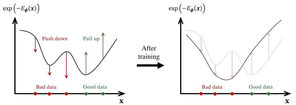
In this view, points with lower energy correspond to higher probability, much like a ball rolling down into a valley. The partition function \(Z_{{\bm{\phi}}}\) ensures that all probabilities add up to one, and as a result only the relative values of energy matter. For instance, adding a constant to all energies multiplies both numerator and denominator by the same factor, leaving the distribution unchanged.
Moreover, because the partition function \(Z_{{\bm{\phi}}}\) enforces that probabilities sum to one, it follows mathematically that decreasing the energy within a region increases its probability, while the probability of its complement decreases accordingly. Thus, EBMs obey a strict global trade-off: making one valley deeper inevitably makes others shallower, and probability mass is redistributed across the entire space rather than assigned independently to each region.
Challenges of Maximum Likelihood Training in EBMs.
In principle, EBMs can be trained by maximum likelihood, which naturally balances fitting the data with global regularization (see Equation in Chapter 1): \[\begin{align} \label{eq:mle-ebm} \mathcal{L}_{\text{MLE}}({\bm{\phi}}) &= \mathbb{E}_{p_{\text{data}}({\mathbf{x}})} \left[ \log \frac{\exp(-E_{{\bm{\phi}}}({\mathbf{x}}))}{Z_{\bm{\phi}}} \right] \\ &= - \underbrace{\mathbb{E}_{p_{\text{data}}}[E_{{\bm{\phi}}}({\mathbf{x}})]}_{\text{lowers energy of data}} - \underbrace{\log \int \exp(-E_{{\bm{\phi}}}({\mathbf{x}}))\mathop{}\!\mathrm{d}{\mathbf{x}}}_{\text{global regularization}}, \nonumber \end{align}\] with \(Z_{\bm{\phi}}= \int \exp(-E_{\bm{\phi}}({\mathbf{x}}))\mathop{}\!\mathrm{d}{\mathbf{x}}\). The first term lowers the energy of real data, while the second enforces normalization via the partition function.
However, in high dimensions computing \(\log Z_{{\bm{\phi}}}\) and its gradient is intractable, as it requires expectations under the model distribution. This motivates alternative objectives that either approximate the term, such as contrastive divergence (Hinton 2002), or avoid it altogether through score matching.
In what follows, we first introduce the notion of the score function in Section 1.1.2 and present score matching as a tractable training objective that bypasses the partition function in Section 1.1.3, and then discuss Langevin dynamics as a practical sampling method with score functions in Section 1.1.4.
Motivation: What Is the Score?
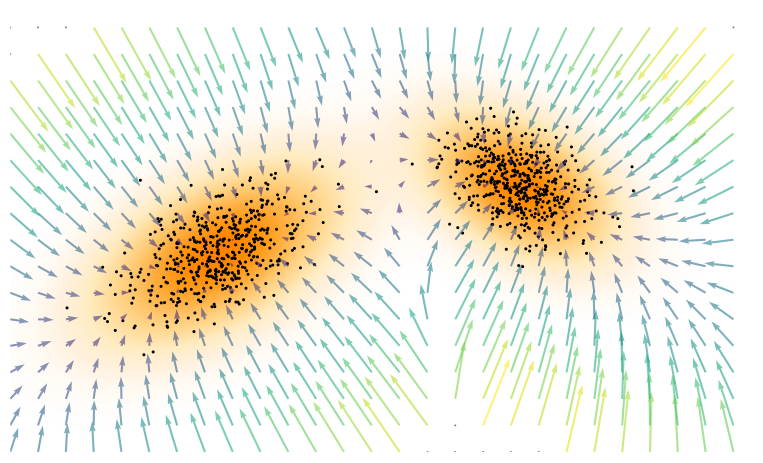
For a density \(p({\mathbf{x}})\) on \(\mathbb{R}^D\), the score function is the gradient of the log-density: \[{\mathbf{s}}({\mathbf{x}}) := \nabla_{{\mathbf{x}}} \log p({\mathbf{x}}), \qquad {\mathbf{s}}\colon \mathbb{R}^D \to \mathbb{R}^D.\] Intuitively, the score forms a vector field that points toward regions of higher probability, providing a local guide to where the data is most likely to occur (see Figure 1.2).
Why Model Scores Instead of Densities?
Modeling the score offers both theoretical and practical benefits:
1. Freedom from Normalization Constants.
Many distributions are defined only up to an unnormalized density \(\tilde{p}({\mathbf{x}})\), e.g., \(\exp(-E_{\bm{\phi}}({\mathbf{x}}))\) in EBMs: \[p({\mathbf{x}}) = \frac{\tilde{p}({\mathbf{x}})}{Z}, \qquad Z = \int \tilde{p}({\mathbf{x}})\mathop{}\!\mathrm{d}{\mathbf{x}}.\] While computing \(Z\) is intractable, the score depends only on \(\tilde{p}\): \[\begin{align} \label{eq:score-compute} \nabla_{{\mathbf{x}}}\log p({\mathbf{x}}) = \nabla_{{\mathbf{x}}}\log \tilde{p}({\mathbf{x}}) - \underbrace{\nabla_{{\mathbf{x}}}\log Z}_{=0} = \nabla_{{\mathbf{x}}}\log \tilde{p}({\mathbf{x}}), \end{align}\] since \(Z\) is constant in \({\mathbf{x}}\). This bypasses the partition function entirely.
2. A Complete Representation.
The score function fully characterizes the underlying distribution. Since it is the gradient of the log-density, the density can be recovered (up to a constant) via \[\log p({\mathbf{x}}) = \log p({\mathbf{x}}_0) + \int_0^1 {\mathbf{s}}({\mathbf{x}}_0 + t({\mathbf{x}}- {\mathbf{x}}_0))^\top ({\mathbf{x}}- {\mathbf{x}}_0) \mathop{}\!\mathrm{d}t,\] where \({\mathbf{x}}_0\) is a reference point and \(\log p({\mathbf{x}}_0)\) is fixed by normalization. Thus, modeling the score is as expressive as modeling \(p({\mathbf{x}})\) itself, while often more tractable for generative modeling.
Training EBMs via Score Matching
In EBMs, the density is defined as \(p_{{\bm{\phi}}}(\mathbf{x}) = \tfrac{\exp(-E_{\bm{\phi}}(\mathbf{x}))}{Z_{\bm{\phi}}}\). Maximum likelihood training requires computing \(Z_{\bm{\phi}}\), which is generally intractable. A key observation is that the model score of \(p_{{\bm{\phi}}}\) simplifies to: \(-\nabla_{{\mathbf{x}}}E_{\bm{\phi}}({\mathbf{x}})\), independent of \(Z_{\bm{\phi}}\) (see Equation \(\eqref{eq:score-compute}\)).
Score matching (Hyvärinen and Dayan 2005) leverages the fact that scores depend only on the energy function. Instead of fitting normalized probabilities, it trains EBMs by aligning the model score with the (unknown) data score: \[\begin{align} \label{eq:ebm-sm} \mathcal{L}_{\mathrm{SM}}(\bm{\phi}) = \tfrac{1}{2} \mathbb{E}_{p_{\mathrm{data}}(\mathbf{x})} \big\| \nabla_{\mathbf{x}} \log p_{\bm{\phi}}(\mathbf{x}) - \nabla_{\mathbf{x}} \log p_{\mathrm{data}}(\mathbf{x}) \big\|_2^2. \end{align}\]
Although the data score is inaccessible, integration by parts yields an equivalent expression involving only the energy and its derivatives (see Proposition: Hyvärinen’s Tractable Form of SM for more details): \[\mathcal{L}_{\mathrm{SM}}(\bm{\phi}) = \mathbb{E}_{p_{\mathrm{data}}(\mathbf{x})} \left[ -\mathop{\mathrm{Tr}}\big(\nabla_{\mathbf{x}}^2 E_{\bm{\phi}}({\mathbf{x}})\big) + \tfrac{1}{2} \|\nabla_{\mathbf{x}} E_{\bm{\phi}}({\mathbf{x}})\|_2^2 \right] + C,\] where \(\nabla_{\mathbf{x}}^2 E_{\bm{\phi}}({\mathbf{x}})\) is the Hessian of \(E_{\bm{\phi}}\) and \(C\) is a constant independent of \(\bm{\phi}\).
This formulation is attractive because it eliminates the partition function and avoids sampling from the model during training. Its main drawback is the need for second-order derivatives: although one only needs the trace of the Hessian (\(\mathop{\mathrm{Tr}}\big(\nabla_{\mathbf{x}}^2 E_{\bm{\phi}}\big)\)), rather than the full Hessian matrix, exact computation of this term generally requires aggregating second-derivative information across input coordinates, so its cost typically increases with the input dimension \(D\). We will revisit approaches to addressing this limitation later in the chapter.
Langevin Sampling with Score Functions
Sampling from EBMs, defined by the energy function \(E_{\bm{\phi}}(\mathbf{x})\), can be performed using Langevin dynamics. We first present the discrete-time Langevin update and then its continuous-time limit as a stochastic differential equation (SDE). Finally, we discuss the physical intuition behind how Langevin dynamics enables efficient exploration of complex energy landscapes.
Discrete-Time Langevin Dynamics.
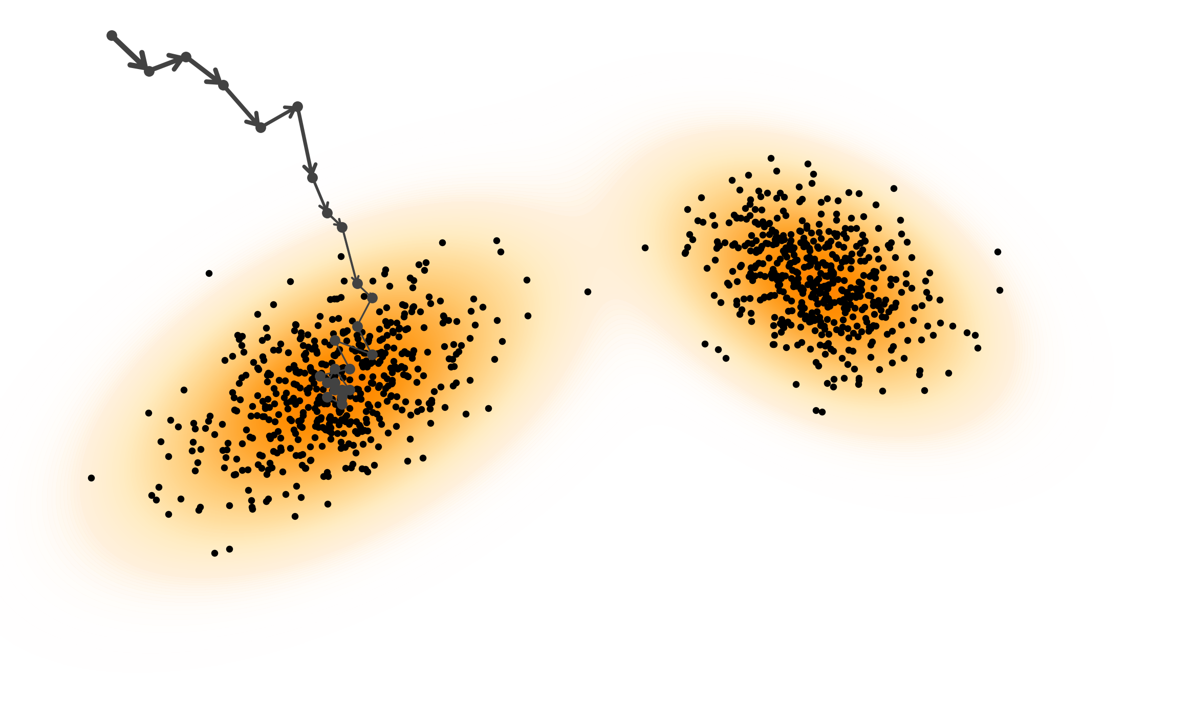
The discrete-time Langevin update is \[\begin{align} \label{eq:discrete-langevin} \mathbf{x}_{n+1} = \mathbf{x}_n - \eta \nabla_{\mathbf{x}} E_{\bm{\phi}}(\mathbf{x}_n) + \sqrt{2 \eta} \bm{\epsilon}_n, \quad n=0,1,2,\ldots, \end{align}\] where \(\mathbf{x}_0\) is initialized from some distribution (often Gaussian), \(\eta > 0\) is the step size, and \(\bm{\epsilon}_n \sim \mathcal{N}(\mathbf{0}, \mathbf{I})\) is Gaussian noise. The noise enables exploration beyond local minima by adding stochasticity.
Since the score function can be computed as \[\nabla_{\mathbf{x}} \log p_{\bm{\phi}}(\mathbf{x}) = -\nabla_{\mathbf{x}} E_{\bm{\phi}}({\mathbf{x}}).\]
the update can equivalently be written as \[\begin{align} \label{eq:discrete-langevin-score} \mathbf{x}_{n+1} = \mathbf{x}_n + \eta \nabla_{\mathbf{x}} \log p_{\bm{\phi}}(\mathbf{x}_n) + \sqrt{2 \eta}\bm{\epsilon}_n, \end{align}\] where the score function guides the samples toward high-density regions. This formulation is central to diffusion models, as will be detailed later.
Continuous-Time Langevin Dynamics.
As the step size \(\eta\) approaches zero, the discrete Langevin updates naturally converge to a continuous-time process described by the Langevin Stochastic Differential Equation (SDE)1 : \[\begin{align} \label{eq:continuous-langevin} \mathop{}\!\mathrm{d}\mathbf{x}(t) = \nabla_{\mathbf{x}} \log p_{\bm{\phi}}(\mathbf{x}(t)) \mathop{}\!\mathrm{d}t + \sqrt{2} \mathop{}\!\mathrm{d}\mathbf{w}(t), \end{align}\] where \(\mathbf{w}(t)\) denotes a standard Brownian motion (also known as a Wiener process2). It is important to understand that the discrete update rule in Equation \(\eqref{eq:discrete-langevin}\) serves as the Euler–Maruyama discretization of this continuous SDE.
Under standard regularity assumptions (e.g., \(p_{\bm{\phi}}\propto e^{-E_{\bm{\phi}}}\) with a confining, sufficiently smooth \(E_{\bm{\phi}}\)), the distribution of \(\mathbf{x}(t)\) converges (exponentially fast) to \(p_{\bm{\phi}}\) as \(t\to\infty\); thus we can sample by simulating (solving) the SDE Equation \(\eqref{eq:continuous-langevin}\).
Why Langevin Sampling?
A natural way to understand Langevin sampling is through the lens of physics, where the energy function \(E_{\bm{\phi}}(\mathbf{x})\) defines a potential landscape that shapes the behavior of particles. According to Newtonian dynamics, the motion of a particle under the force field derived from this energy is described by the ordinary differential equation (ODE) \[\mathop{}\!\mathrm{d}\mathbf{x}(t) = -\nabla_{\mathbf{x}} E_{\bm{\phi}}\big(\mathbf{x}(t)\big) \mathop{}\!\mathrm{d}t,\] which deterministically drives the particle downhill toward a local minimum of the energy function. However, such deterministic dynamics can become trapped in local minima, preventing exploration of the full data distribution.
To overcome this limitation, Langevin dynamics introduces stochastic perturbations, resulting in the SDE \[\mathop{}\!\mathrm{d}\mathbf{x}(t) = -\nabla_{\mathbf{x}} E_{\bm{\phi}}\big(\mathbf{x}(t)\big) \mathop{}\!\mathrm{d}t + \underbrace{\sqrt{2 } \mathop{}\!\mathrm{d}{\mathbf{w}}(t)}_{\text{injected noise}},\] where \({\mathbf{w}}(t)\) is a standard Brownian motion.
The noise term allows the particle to escape local minima by crossing energy barriers, making the trajectory a stochastic process whose stationary distribution converges to the Boltzmann distribution \[p_{\bm{\phi}}(\mathbf{x}) \propto e^{-E_{\bm{\phi}}(\mathbf{x})}.\]
From this perspective, EBMs can be viewed as learning a force field that pushes samples toward regions of high probability. Langevin sampling is particularly useful for EBMs because it provides a practical method to generate samples from the model distribution \(p_{\bm{\phi}}(\mathbf{x})\) without explicitly computing the partition function. By iteratively applying the Langevin update, one obtains samples that approximate the target distribution.
Inherent Challenges of Langevin Sampling.
Langevin dynamics, a widely used MCMC-based sampler, faces serious limitations in high-dimensional spaces. Its efficiency is highly sensitive to the choice of step size \(\eta\), noise scale, and the number of iterations required to approximate the target distribution accurately.
At the heart of this inefficiency lies the issue of poor “mixing time”: In complex data distributions with many isolated modes, Langevin sampling often requires an extremely long time to transition between regions of high probability. This problem becomes significantly worse as dimensionality increases, leading to prohibitively slow convergence.
One can think of sampling as exploring a vast and rugged landscape with many distant valleys, each corresponding to a different data mode. Langevin dynamics, relying on local stochastic updates, struggles to traverse between these valleys efficiently. As a result, it often fails to capture the full diversity of the distribution.
This inefficiency hints the need for more structured and guided sampling methods that can navigate complex data manifolds more effectively than purely random exploration.
From Energy-Based to Score-Based Generative Models
EBMs show that generation depends only on the score, which points toward regions of higher probability, rather than on the full normalized density. While score matching avoids the partition function, training through the energy still requires expensive second derivatives. The key idea is that since sampling with Langevin dynamics needs only the score, we can learn it directly with a neural network. This shift, from modeling energies to modeling scores, forms the foundation of score-based generative models.
Training with Score Matching
Score Matching.
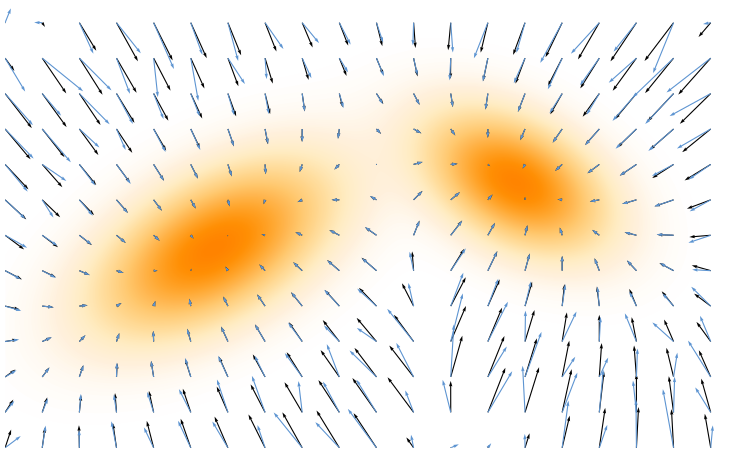
To approximate the score function \({\mathbf{s}}({\mathbf{x}}) = \nabla_{{\mathbf{x}}} \log p_{\mathrm{data}}({\mathbf{x}})\) from samples of \(p_{\mathrm{data}}\), we approximate it directly as a vector field parameterized by a neural network \({\mathbf{s}}_{\bm{\phi}}({\mathbf{x}})\) (see Figure 1.4): \[{\mathbf{s}}_{\bm{\phi}}({\mathbf{x}}) \approx {\mathbf{s}}({\mathbf{x}}).\] Score matching fits this vector field by minimizing the mean squared error (MSE) between the true and estimated scores:
\[\begin{align} \label{eq:sm} \mathcal{L}_{\mathrm{SM}}(\bm{\phi}) := \frac{1}{2} \mathbb{E}_{{\mathbf{x}}\sim p_{\mathrm{data}}} \Big[\| {\mathbf{s}}_{\bm{\phi}}({\mathbf{x}}) - {\mathbf{s}}({\mathbf{x}})\|_2^2\Big]. \end{align}\]
Tractable Score Matching.
At first glance, this objective seems infeasible because the true score \({\mathbf{s}}({\mathbf{x}})\), which serves as the regression target, is unknown. Fortunately, Hyvärinen and Dayan (2005) showed that integration by parts yields an equivalent objective that depends only on the model \({\mathbf{s}}_{\bm{\phi}}\) and the data samples, without requiring access to the true score. We state this key result in the following proposition:
Proposition: Hyvärinen’s Tractable Form of SM
We can express the following equation as: \[\begin{align*} \mathcal{L}_{\text{SM}}(\bm{\phi}) = \widetilde{\mathcal{L}}_{\text{SM}}(\bm{\phi}) + C. \end{align*}\] where \[\begin{align} \label{eq:sm-alternative} \widetilde{\mathcal{L}}_{\text{SM}}(\bm{\phi}) := \mathbb{E}_{{\mathbf{x}}\sim p_{\text{data}}({\mathbf{x}})} \left[ \mathop{\mathrm{Tr}}\left(\nabla_{{\mathbf{x}}}{\mathbf{s}}_{\bm{\phi}}({\mathbf{x}})\right) + \frac{1}{2} \left\lVert{\mathbf{s}}_{\bm{\phi}}({\mathbf{x}})\right\rVert_2^2 \right]. \end{align}\] and \(C\) is a constant that does not depend on \(\bm{\phi}\). The minimizer \({\mathbf{s}}^*\) is obtained as: \({\mathbf{s}}^*(\cdot) = \nabla_{{\mathbf{x}}} \log p(\cdot)\).
Proof for Proposition. The result follows by expanding the MSE in \(\mathcal{L}_{\text{SM}}\) and applying integration by parts. The proof is given in Section (Tractable Score Matching via Integration by Parts) in Appendix D. ■
Using the equivalent objective in Equation \(\eqref{eq:sm-alternative}\), we train the score model \({\mathbf{s}}_{\bm{\phi}}({\mathbf{x}})\) solely from observed samples of \(p_{\mathrm{data}}\), eliminating the need for the true score function.
Intuition of Equation \(\eqref{eq:sm-alternative}\).
The alternative score matching objective \(\widetilde{\mathcal{L}}_{\text{SM}}(\bm\phi)\) can be understood from its two terms. The norm term \(\tfrac12\|{\mathbf{s}}_{\bm\phi}({\mathbf{x}})\|^2\) penalizes large score values, especially in regions where \(p_{\mathrm{data}}\) is large. The divergence term \(\mathop{\mathrm{Tr}}(\nabla_{{\mathbf{x}}} {\mathbf{s}}_{\bm\phi}({\mathbf{x}}))\) appears with a positive sign in the loss, so minimizing the objective also favors locally contracting behavior. Together, these two terms yield the population-optimal score field \({\mathbf{s}}^*({\mathbf{x}})=\nabla_{{\mathbf{x}}}\log p_{\mathrm{data}}({\mathbf{x}})\). We explain the geometric intuition in more detail below.
Effect of the Magnitude Term.
Since the expectation in \(\widetilde{\mathcal{L}}_{\mathrm{SM}}(\bm\phi)\) is taken under \(p_{\mathrm{data}}\), regions where \(p_{\mathrm{data}}({\mathbf{x}})\) is large (high data density) contribute more strongly to the loss. The magnitude term \(\tfrac12\|{\mathbf{s}}_{\bm\phi}({\mathbf{x}})\|^2\) therefore places a stronger penalty on large score values in these regions. By itself, however, this term does not imply that \({\mathbf{s}}_{\bm\phi}({\mathbf{x}})=\mathbf{0}\) at every high-density point; at the population optimum, \[{\mathbf{s}}^*({\mathbf{x}})=\nabla_{{\mathbf{x}}}\log p_{\mathrm{data}}({\mathbf{x}}),\] which vanishes only at stationary points of the log-density.
Concavity When the Field is (Approximately) a Gradient.
Because the divergence term \(\mathop{\mathrm{Tr}}(\nabla_{{\mathbf{x}}} {\mathbf{s}}_{\bm\phi}({\mathbf{x}}))\) enters the loss with a positive sign, minimizing the objective favors negative divergence in regions emphasized by the data distribution. Negative divergence indicates net local contraction, although by itself it does not guarantee that a stationary point is a sink. To make this precise, assume \({\mathbf{s}}_{\bm\phi}=\nabla_{{\mathbf{x}}}u\) for a scalar function \(u:\mathbb{R}^D\to\mathbb{R}\), as is natural when matching a log density. Then \(\nabla_{{\mathbf{x}}}{\mathbf{s}}_{\bm\phi}=\nabla_{{\mathbf{x}}}^2 u\) (the Hessian) and \(\nabla \cdot {\mathbf{s}}_{\bm\phi}({\mathbf{x}})=\mathop{\mathrm{Tr}}(\nabla_{{\mathbf{x}}}^2 u({\mathbf{x}}))\) (the divergence).
At a stationary point \({\mathbf{x}}_\star\), where \({\mathbf{s}}_{\bm\phi}({\mathbf{x}}_\star)=\nabla_{{\mathbf{x}}}u({\mathbf{x}}_\star)=\mathbf{0}\), a second order Taylor expansion gives \[u({\mathbf{x}}) = u({\mathbf{x}}_\star) + \tfrac12({\mathbf{x}}-{\mathbf{x}}_\star)^\top \nabla_{{\mathbf{x}}}^2 u({\mathbf{x}}_\star)({\mathbf{x}}-{\mathbf{x}}_\star) + o(\|{\mathbf{x}}-{\mathbf{x}}_\star\|^2).\] If the Hessian \(\nabla_{{\mathbf{x}}}^2 u({\mathbf{x}}_\star)\) is negative definite, then \(u\) is locally concave at \({\mathbf{x}}_\star\) and the log density attains a strict local maximum3 there. Because all eigenvalues of the Hessian are negative, the trace is also negative: \(\mathop{\mathrm{Tr}}(\nabla_{{\mathbf{x}}}^2 u({\mathbf{x}}_\star))<0\). Thus, in this case, the stationary point is locally attracting under the score field: small perturbations are pulled back toward \({\mathbf{x}}_\star\).
Sampling with Langevin Dynamics
Once trained by minimizing Equation \(\eqref{eq:sm-alternative}\), the score model \({\mathbf{s}}_{\bm{\phi}^\times}({\mathbf{x}})\) can replace the oracle score in Langevin dynamics for sampling: \[\begin{align} \label{eq:score-langevin-emp} \mathbf{x}_{n+1} = \mathbf{x}_n + \eta {\mathbf{s}}_{\bm{\phi}^\times}({\mathbf{x}}_n) + \sqrt{2\eta} \bm{\epsilon}_n, \quad \bm{\epsilon}_n \sim \mathcal{N}(\bm{0}, \bm{I}), \end{align}\] for \(n=0,1,2,\dots\), initialized at \({\mathbf{x}}_0\). As in the EBM case Equation \(\eqref{eq:continuous-langevin}\), this recursion is precisely the Euler–Maruyama discretization of the continuous-time Langevin SDE: \[\begin{align*} \mathop{}\!\mathrm{d}{\mathbf{x}}(t) = {\mathbf{s}}_{\bm{\phi}^\times}({\mathbf{x}}(t)) \mathop{}\!\mathrm{d}t + \sqrt{2} \mathop{}\!\mathrm{d}\mathbf{w}(t), \end{align*}\] with initialization \({\mathbf{x}}(0)\). Hence, in the limit of small step size, the discrete and continuous formulations coincide. In practice, one can either run the discrete sampler or directly simulate the SDE.
Prologue: Score-Based Generative Models
In the remainder of this chapter, we examine the foundational role of the score function in modern diffusion models. Initially introduced to enable efficient training of EBMs, the score function has evolved into a central component of a new generation of generative models. Building on this foundation, we explore how the score function informs the theoretical formulation and practical implementation of score-based diffusion models, offering a principled framework for data generation via stochastic processes.
Denoising Score Matching
Motivation
Although the alternative objective in Equation \(\eqref{eq:sm-alternative}\) \[\begin{align*} \widetilde{\mathcal{L}}_{\text{SM}}(\bm{\phi}) = \mathbb{E}_{{\mathbf{x}}\sim p_{\mathrm{data}}} \left[\mathrm{Tr}\big(\nabla_{{\mathbf{x}}}{\mathbf{s}}_{\bm{\phi}}({\mathbf{x}})\big) + \frac{1}{2} \|{\mathbf{s}}_{\bm{\phi}}({\mathbf{x}})\|_2^2 \right] \end{align*}\] is more tractable, it still requires computing the trace of the Jacobian, \(\mathrm{Tr}(\nabla_{{\mathbf{x}}}{\mathbf{s}}_{\bm{\phi}}({\mathbf{x}}))\). Although this does not require forming the full Jacobian matrix, exact evaluation generally becomes more expensive as the input dimension \(D\) increases, since it requires aggregating derivative information across input coordinates. This can therefore be computationally expensive in high dimensions.
To address this, sliced score matching (Song et al. 2020) replaces the trace term with a stochastic estimate based on random projections. We briefly outline the idea below.
Sliced Score Matching and Hutchinson’s Estimator.
Sliced score matching replaces the trace in score matching by averaging directional derivatives along random “slices”. Let \({\mathbf{u}}\in\mathbb{R}^D\) be an isotropic random vector (e.g., Rademacher or standard Gaussian) with \(\mathbb{E}[{\mathbf{u}}]=0\) and \(\mathbb{E}[{\mathbf{u}}{\mathbf{u}}^\top]=\mathbf I\). By Hutchinson’s identity \[\mathop{\mathrm{Tr}}({\mathbf{A}})=\mathbb{E}_{{\mathbf{u}}}[{\mathbf{u}}^\top {\mathbf{A}}{\mathbf{u}}],\quad\text{and}\quad\mathbb{E}_{{\mathbf{u}}}[({\mathbf{u}}^\top{\mathbf{s}}_{{\bm{\phi}}}({\mathbf{x}}))^2]=\|{\mathbf{s}}_{{\bm{\phi}}}({\mathbf{x}})\|_2^2,\] we obtain the exact form \[\widetilde{\mathcal{L}}_{\mathrm{SM}}({\bm{\phi}}) =\mathbb{E}_{{\mathbf{x}},{\mathbf{u}}} \Big[{\mathbf{u}}^\top\big(\nabla_{{\mathbf{x}}}{\mathbf{s}}_{{\bm{\phi}}}({\mathbf{x}})\big){\mathbf{u}}+\tfrac12({\mathbf{u}}^\top{\mathbf{s}}_{{\bm{\phi}}}({\mathbf{x}}))^2\Big].\] This objective can be evaluated efficiently with automatic differentiation, using Jacobian- and vector-Jacobian-product operations (JVP/VJP) instead of explicitly computing large Jacobian or Hessian matrices. Averaging over \(K\) random probes yields an unbiased estimator with variance \(\mathcal{O}(1/K)\), and the directional term \({\mathbf{u}}^\top(\nabla_{{\mathbf{x}}}{\mathbf{s}}_{{\bm{\phi}}}){\mathbf{u}}\) can be computed efficiently using JVP/VJP routines without explicit Jacobians. Intuitively, this means we only check the model’s behavior along random directions: the projected score is nudged to align with regions of higher data density, so data points become stationary in expectation.
From Sliced to Denoising Score Matching.
Sliced score matching sidesteps Jacobians but still relies on the raw data distribution. This makes it fragile: for image data lying on low-dimensional manifolds, the score \(\nabla_{{\mathbf{x}}}\log p_{\mathrm{data}}({\mathbf{x}})\) may be undefined or unstable, and the method only constrains the vector field at observed points, providing weak control in their neighborhoods. It further suffers from probe-induced variance and repeated JVP/VJP costs.
A more robust alternative, which we focus on here, is Denoising Score Matching (DSM) (Vincent 2011), which offers a principled and scalable solution.
Training
Let us revisit the SM loss in Equation \(\eqref{eq:sm}\): \[\begin{align*} \mathcal{L}_{\text{SM}}(\bm{\phi}) = \frac{1}{2} \mathbb{E}_{{\mathbf{x}}\sim p_{\text{data}}({\mathbf{x}})} \left[ \left\lVert{\mathbf{s}}_{\bm{\phi}}({\mathbf{x}}) - \nabla_{{\mathbf{x}}} \log p_{\text{data}}({\mathbf{x}})\right\rVert_2^2 \right], \end{align*}\] where the issue arises from the intractable term \(\nabla_{{\mathbf{x}}} \log p_{\text{data}}({\mathbf{x}})\).
Vincent (2011)’s Solution by Conditioning.
To overcome the intractability of \(\nabla_{{\mathbf{x}}} \log p_{\text{data}}({\mathbf{x}})\), Vincent (2011) proposed injecting noise into the data \({\mathbf{x}}\sim p_{\text{data}}\) via a known conditional distribution \(p_{\sigma}(\tilde{{\mathbf{x}}}|{\mathbf{x}})\) with scale \(\sigma\). The neural network \({\mathbf{s}}_{\bm{\phi}}(\tilde{{\mathbf{x}}}, \sigma)\) is trained to approximate the score of the marginal perturbed distribution \[p_\sigma(\tilde{{\mathbf{x}}}) = \int p_{\sigma}(\tilde{{\mathbf{x}}}|{\mathbf{x}}) p_{\text{data}}({\mathbf{x}}) \mathop{}\!\mathrm{d}{\mathbf{x}}\] by minimizing the loss \[\begin{align} \label{eq:sm-noise-loss} \mathcal{L}_{\text{SM}}(\bm{\phi}; \sigma) := \frac{1}{2} \mathbb{E}_{\tilde{{\mathbf{x}}} \sim p_\sigma} \left[ \left\lVert{\mathbf{s}}_{\bm{\phi}}(\tilde{{\mathbf{x}}}, \sigma) - \nabla_{\tilde{{\mathbf{x}}}} \log p_\sigma(\tilde{{\mathbf{x}}})\right\rVert_2^2 \right]. \end{align}\]
Even though \(\nabla_{\tilde{{\mathbf{x}}}} \log p_\sigma(\tilde{{\mathbf{x}}})\) is generally intractable, Vincent (2011) showed that conditioning on \({\mathbf{x}}\sim p_{\text{data}}\) yields an equivalent, tractable objective—the Denoising Score Matching (DSM) loss:
\[\begin{align} \label{eq:dsm-loss} \mathcal{L}_{\text{DSM}}(\bm{\phi}; \sigma) := \frac{1}{2} \mathbb{E}_{{\mathbf{x}}\sim p_{\text{data}}, \tilde{{\mathbf{x}}} \sim p_{\sigma}(\cdot|{\mathbf{x}})} \left[ \left\lVert{\mathbf{s}}_{\bm{\phi}}(\tilde{{\mathbf{x}}}, \sigma) - \nabla_{\tilde{{\mathbf{x}}}} \log p_{\sigma}(\tilde{{\mathbf{x}}}|{\mathbf{x}})\right\rVert_2^2 \right]. \end{align}\]
The optimal minimizer \({\mathbf{s}}^*\) of Equation \(\eqref{eq:dsm-loss}\) satisfies \[{\mathbf{s}}^*(\tilde{{\mathbf{x}}}, \sigma) = \nabla_{\tilde{{\mathbf{x}}}} \log p_\sigma(\tilde{{\mathbf{x}}}),\] which is also optimal for Equation \(\eqref{eq:sm-noise-loss}\).
For example, when \(p_{\sigma}(\tilde{{\mathbf{x}}}|{\mathbf{x}})\) is Gaussian noise with variance \(\sigma^2\), \[p_{\sigma}(\tilde{{\mathbf{x}}}|{\mathbf{x}}) = \mathcal{N}(\tilde{{\mathbf{x}}}; {\mathbf{x}}, \sigma^2 \mathbf{I}),\] the gradient \(\nabla_{\tilde{{\mathbf{x}}}} \log p_{\sigma}(\tilde{{\mathbf{x}}}|{\mathbf{x}})\) has a closed form (see Equation \(\eqref{eq:gaussian-dsm}\)), making the regression target explicit and computationally tractable.
Moreover, as \(\sigma \approx 0\), \(p_\sigma(\tilde{{\mathbf{x}}}) \approx p_{\text{data}}({\mathbf{x}})\) and \[{\mathbf{s}}^*(\tilde{{\mathbf{x}}}, \sigma) = \nabla_{\tilde{{\mathbf{x}}}} \log p_\sigma(\tilde{{\mathbf{x}}}) \approx \nabla_{{\mathbf{x}}} \log p_{\text{data}}({\mathbf{x}}),\] indicating the learned score approximates the original data score, enabling its use in generation.
We formalize this discussion on the gradient equivalence between \(\mathcal{L}_{\text{SM}}\) and \(\mathcal{L}_{\text{DSM}}\) in the following theorem:
Theorem: Equivalence of \(\mathcal{L}_{\text{SM}}\) and \(\mathcal{L}_{\text{DSM}}\)
For any fixed noise scale \(\sigma > 0\), the following holds: \[\begin{align} \label{eq:score-matching} \mathcal{L}_{\text{SM}}(\bm{\phi}; \sigma) = \mathcal{L}_{\text{DSM}}(\bm{\phi}; \sigma) + C, \end{align}\] where \(C\) is a constant independent of the parameter \(\bm{\phi}\). Furthermore, the minimizer \({\mathbf{s}}^*(\cdot, \sigma)\) of both losses satisfies \[{\mathbf{s}}^*(\tilde{{\mathbf{x}}}, \sigma) = \nabla_{\tilde{{\mathbf{x}}}} \log p_\sigma(\tilde{{\mathbf{x}}}), \quad \text{for almost every } \tilde{{\mathbf{x}}}.\]
Proof for Theorem. The equivalence follows from a
direct computation: by expanding the MSE in \(\mathcal{L}_{\text{SM}}\) and \(\mathcal{L}_{\text{DSM}}\), all \(\bm{\phi}\)-dependent terms cancel, leaving
only a constant difference independent of \(\bm{\phi}\).
The derivation of the minimizer follows the same argument as in
Proposition in Chapter 4 (Minimizer of DSM). We defer the
detailed derivation to Section (Equivalence Between SM and DSM Minimization) in Appendix D. ■
This theorem, like Theorem in Chapter 2 (Equivalence Between Marginal and Conditional KL Minimization) in DDPM, illustrates a key shared principle:
Insight: Conditioning Technique
The conditioning technique also appears in the variational view of diffusion models in DDPM (see Theorem in Chapter 2 (Equivalence Between Marginal and Conditional KL Minimization)), where conditioning on a data point \({\mathbf{x}}\) turns an intractable loss into a tractable one for Monte Carlo estimation. A similar idea arises in the flow-based perspective (e.g., Flow Matching (Lipman et al. 2022)), as we will see in Section (Flow Matching FrameworkFlow Matching Framework) in Chapter 5.
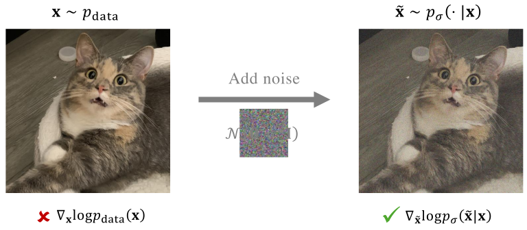
Special Case: Additive Gaussian Noise.
We now consider the common case where Gaussian noise \(\mathcal{N}(\mathbf{0}, \sigma^2 {\mathbf{I}})\) with variance \(\sigma^2\) is added to each data point \({\mathbf{x}}\sim p_{\text{data}}\): \[\tilde{{\mathbf{x}}} = {\mathbf{x}}+ \sigma \bm{\epsilon}, \quad \bm{\epsilon} \sim \mathcal{N}(\mathbf{0}, {\mathbf{I}}),\] so that the corrupted data \(\tilde{{\mathbf{x}}}\) follows \[p_{\sigma}(\tilde{{\mathbf{x}}}|{\mathbf{x}}) = \mathcal{N}(\tilde{{\mathbf{x}}}; {\mathbf{x}}, \sigma^2 {\mathbf{I}}).\] In this setting, the conditional score is analytically given by \[\nabla_{\tilde{{\mathbf{x}}}} \log p_{\sigma}(\tilde{{\mathbf{x}}}|{\mathbf{x}}) = \frac{{\mathbf{x}}- \tilde{{\mathbf{x}}}}{\sigma^2}.\] Hence, the DSM loss simplifies to:
\[\begin{align} \label{eq:gaussian-dsm} \begin{aligned} \mathcal{L}_{\text{DSM}}(\bm{\phi}; \sigma) &= \frac{1}{2} \mathbb{E}_{{\mathbf{x}}, \tilde{{\mathbf{x}}}|{\mathbf{x}}} \left[ \left\lVert{\mathbf{s}}_{\bm{\phi}}(\tilde{{\mathbf{x}}}, \sigma) - \frac{{\mathbf{x}}- \tilde{{\mathbf{x}}}}{\sigma^2}\right\rVert_2^2 \right] \\ &= \frac{1}{2} \mathbb{E}_{{\mathbf{x}}, \bm{\epsilon}} \left[ \left\lVert{\mathbf{s}}_{\bm{\phi}}({\mathbf{x}}+ \sigma \bm{\epsilon}, \sigma) + \frac{\bm{\epsilon}}{\sigma}\right\rVert_2^2 \right], \end{aligned} \end{align}\]
where \(\bm{\epsilon} \sim \mathcal{N}(\mathbf{0}, {\mathbf{I}})\). This objective forms the core of the (score-based) Diffusion Model.
At a fixed noise level \(\sigma>0\), DSM learns the score of the Gaussian-smoothed distribution \[p_\sigma = p_{\mathrm{data}} * \mathcal{N}(\bm{0},\sigma^2{\mathbf{I}}),\] rather than the score of \(p_{\mathrm{data}}\) itself. When \(\sigma\) is small, the corruption is mild, so \(p_\sigma\) still closely preserves the local structure of the data distribution. Its score therefore provides a useful direction for moving noisy samples back toward likely data regions. As \(\sigma\) becomes larger, the Gaussian smoothing progressively removes fine details and merges nearby modes. The corresponding score then captures mainly coarser, more global structure. This behavior is useful rather than undesirable: the multi-noise construction in Section 1.4 deliberately combines many noise levels, using large noise for coarse exploration and small noise for fine refinement.
To better see why the objective naturally corresponds to a “denoising” process, we expand on the discussion in Section (Why DSM is Denoising: Tweedie’s Formula) and Section ((Optional) Why DSM is Denoising: SURE).
Sampling
Once we have a trained score model \({\mathbf{s}}_{\bm{\phi}^\times}(\tilde{{\mathbf{x}}}, \sigma)\) at noise level \(\sigma\), we generate samples using Langevin dynamics by replacing the true score with the learned model. The update rule is: \[\begin{align} \label{eq:score-langevin-emp-dsm} \tilde{{\mathbf{x}}}_{n+1} = \tilde{{\mathbf{x}}}_n + \eta \underbrace{{\mathbf{s}}_{\bm{\phi}^\times}(\tilde{{\mathbf{x}}}_n, \sigma)}_{\approx \nabla_{\tilde{{\mathbf{x}}}} \log p_\sigma(\tilde{{\mathbf{x}}}_n)} + \sqrt{2\eta} \bm{\epsilon}_n, \quad \bm{\epsilon}_n \sim \mathcal{N}(\mathbf{0}, {\mathbf{I}}), \end{align}\] for \(n = 0, 1, 2, \dots\), starting from an initial value \(\tilde{{\mathbf{x}}}_0\). If \(\sigma\) is sufficiently small, then after enough iterations, \(\tilde{{\mathbf{x}}}_n\) approximates samples from \(p_{\text{data}}\).
Advantages of Noise Injection.
We additionally remark that, compared to vanilla score matching in Equation \(\eqref{eq:sm}\), injecting Gaussian noise to form \(p_\sigma\) (e.g., Equation \(\eqref{eq:gaussian-dsm}\)) provides two key advantages (Song and Ermon 2019):
Well-Defined Gradients. The noise perturbs data away from its lower-dimensional manifold, resulting in a distribution \(p_\sigma\) with full support in \(\mathbb{R}^D\). Consequently, the score function \(\nabla_{\tilde{{\mathbf{x}}}} \log p_\sigma(\tilde{{\mathbf{x}}})\) is well-defined everywhere.
Improved Coverage. The noise smooths out sparse regions between modes, enhancing training signal quality and facilitating Langevin dynamics to traverse low-density regions more effectively.
Why DSM is Denoising: Tweedie’s Formula
We begin with Tweedie’s formula (Efron 2011), which provides a principled basis for denoising from noisy observations alone. Concretely, it states that: given a single Gaussian–corrupted observation \(\tilde{{\mathbf{x}}}\sim\mathcal N(\,\cdot\,;\alpha{\mathbf{x}},\sigma^2\mathrm{I})\) from an unknown \({\mathbf{x}}\sim p_{\mathrm{data}}\), a denoised estimate (the average over all plausible clean signals given \(\tilde{{\mathbf{x}}}\)) is obtained by nudging \(\tilde{{\mathbf{x}}}\) a step of size \(\sigma^2\) in the direction of the score \(\nabla_{\tilde{{\mathbf{x}}}}\log p_\sigma(\tilde{{\mathbf{x}}})\) of its noisy marginal defined as: \[p_\sigma(\tilde{{\mathbf{x}}}):= \int \mathcal{N}(\tilde{{\mathbf{x}}};\alpha {\mathbf{x}},\sigma^2\mathrm{I})p_{\mathrm{data}}({\mathbf{x}})\mathop{}\!\mathrm{d}{\mathbf{x}}.\] We present the proposition formally below.
Lemma: Tweedie’s Formula
Assume \({\mathbf{x}}\sim p_{\mathrm{data}}\) and, conditionally on \({\mathbf{x}}\), \(\tilde{{\mathbf{x}}}\sim\mathcal N(\,\cdot\,;\alpha{\mathbf{x}},\sigma^2\mathrm{I})\) with \(\alpha\neq 0\). Then Tweedie’s formula states \[\begin{align} \label{eq:tweedie} \alpha \mathbb{E}_{{\mathbf{x}}\sim p({\mathbf{x}}|\tilde{\mathbf{x}})}\big[{\mathbf{x}}\big| \tilde{\mathbf{x}}\big] = \tilde{\mathbf{x}}+ \sigma^2 \nabla_{\tilde{\mathbf{x}}} \log p_\sigma(\tilde{\mathbf{x}}), \end{align}\] where the expectation is taken over the posterior distribution \(p({\mathbf{x}}|\tilde{\mathbf{x}})\) of \({\mathbf{x}}\) given \(\tilde{\mathbf{x}}\).
Proof for Lemma. The proof proceeds by computing the score of the marginal \[p(\tilde{\mathbf{x}})=\int p(\tilde{\mathbf{x}}|{\mathbf{x}})p_{\mathrm{data}}({\mathbf{x}})\mathop{}\!\mathrm{d}{\mathbf{x}}.\] Differentiating under the integral and using the Gaussian form of the conditional density leads directly to an expression that rearranges into the desired identity linking the score with the posterior mean. See Section (Tweedie’s Formula) in Appendix D for details. ■
Tweedie’s formula plays a central role in diffusion models, where multiple layers of noise are introduced as in DDPM. It enables the estimation of clean samples from noisy observations via the score function, thereby establishing a fundamental link between score prediction and denoiser: \[\begin{equation*} \underbrace{\mathbb{E} \left[{\mathbf{x}}|\tilde{\mathbf{x}}\right]}_{\substack{\text{denoiser}\\\ text{estimated from }\tilde{\mathbf{x}}}} = \frac{1}{\alpha}\left(\tilde{\mathbf{x}}+ \sigma^2 \nabla_{\tilde{\mathbf{x}}} \log p_\sigma(\tilde{\mathbf{x}})\right). \end{equation*}\]
Especially, a single gradient-ascent step on the noisy log-likelihood with the particular step size \(\sigma^2\) is the denoised estimate (the conditional average clean signal). This makes DSM training and denoising tightly related: if \({\mathbf{s}}_{\bm{\phi}}(\tilde{{\mathbf{x}}})\approx \nabla_{\tilde{{\mathbf{x}}}}\log p_\sigma(\tilde{{\mathbf{x}}})\) trained from DSM, then \[\frac{1}{\alpha}\left(\tilde{{\mathbf{x}}}+\sigma^2 {\mathbf{s}}_{\bm{\phi}}(\tilde{{\mathbf{x}}})\right)\] is the denoiser.
(Optional) Higher Order Tweedie’s Formula.
The classical Tweedie’s formula expresses the posterior mean \(\mathbb{E}[{\mathbf{x}}_0|\tilde{{\mathbf{x}}}]\) through the gradient \(\nabla_{\tilde{{\mathbf{x}}}}\log p(\tilde{{\mathbf{x}}})\). Higher order extensions (Meng et al. 2021) express the posterior covariance and higher cumulants through higher derivatives of \(\log p(\tilde{{\mathbf{x}}})\).
Exponential Family Setup with the Log-Normalizer \(\lambda(\tilde{{\mathbf{x}}})\).
Assume the conditional law of \(\tilde{{\mathbf{x}}}\) given a latent natural parameter \(\boldsymbol\eta\in\mathbb{R}^D\) belongs to a natural exponential family written as \[q_\sigma(\tilde{{\mathbf{x}}}|\boldsymbol\eta) =\exp\!\big(\boldsymbol\eta^\top \tilde{{\mathbf{x}}}-\psi(\boldsymbol\eta)\big)\,q_0(\tilde{{\mathbf{x}}}).\] Here \(q_0(\tilde{{\mathbf{x}}})\) is the base measure, namely the part that does not depend on \(\boldsymbol\eta\); for additive Gaussian noise with variance \(\sigma^2{\mathbf{I}}\) it equals \((2\pi\sigma^2)^{-D/2}\exp(-\|\tilde{{\mathbf{x}}}\|^2/2\sigma^2)\). Let \(p(\boldsymbol\eta)\) be the pre-defined distribution of the latent natural parameter, which can be viewed as the reparameterized clean-data distribution (for Gaussian location, \(\boldsymbol\eta={\mathbf{x}}/\sigma^2\)). The observed noisy marginal is \[p_\sigma(\tilde{{\mathbf{x}}})=\int q_\sigma(\tilde{{\mathbf{x}}}|\boldsymbol\eta)\,p(\boldsymbol\eta)\mathop{}\!\mathrm{d}\boldsymbol\eta.\] Define the log-partition (log-normalizer) in \(\tilde{{\mathbf{x}}}\) by \[\lambda(\tilde{{\mathbf{x}}}) := \log p_\sigma(\tilde{{\mathbf{x}}})-\log q_0(\tilde{{\mathbf{x}}}).\] Then the posterior of \(\boldsymbol\eta\) given \(\tilde{{\mathbf{x}}}\) is \[p(\boldsymbol\eta|\tilde{{\mathbf{x}}}) \ \propto\ \exp\!\big(\boldsymbol\eta^\top \tilde{{\mathbf{x}}}-\psi(\boldsymbol\eta)-\lambda(\tilde{{\mathbf{x}}})\big)\,p(\boldsymbol\eta),\] which shows that, as a function of \(\tilde{{\mathbf{x}}}\), the posterior has exponential-family form with natural parameter \(\tilde{{\mathbf{x}}}\), sufficient statistic \(\boldsymbol\eta\), and log-partition \(\lambda(\tilde{{\mathbf{x}}})\).
Derivatives of \(\lambda\) Produce Posterior Cumulants.
Two simple rules are at play. First, normalization: for every \(\tilde{{\mathbf{x}}}\), \[\int \exp\!\big(\boldsymbol\eta^\top \tilde{{\mathbf{x}}}-\psi(\boldsymbol\eta)-\lambda(\tilde{{\mathbf{x}}})\big)\,p(\boldsymbol\eta)\mathop{}\!\mathrm{d}\boldsymbol\eta =1.\] Differentiating this identity with respect to \(\tilde{{\mathbf{x}}}\) brings down powers of \(\boldsymbol\eta\) from the exponential and derivatives of \(\lambda(\tilde{{\mathbf{x}}})\); setting the result to zero yields equalities between derivatives of \(\lambda\) and posterior moments of \(\boldsymbol\eta\). Second, a standard property of exponential families: the log-partition is the cumulant generating function of the sufficient statistic. Therefore \[\nabla_{\tilde{{\mathbf{x}}}}\lambda(\tilde{{\mathbf{x}}})=\mathbb{E}[\boldsymbol\eta|\tilde{{\mathbf{x}}}],\quad \nabla_{\tilde{{\mathbf{x}}}}^{2}\lambda(\tilde{{\mathbf{x}}})=\mathrm{Cov}[\boldsymbol\eta|\tilde{{\mathbf{x}}}],\quad \nabla_{\tilde{{\mathbf{x}}}}^{(k)}\lambda(\tilde{{\mathbf{x}}})=\kappa_k(\boldsymbol\eta|\tilde{{\mathbf{x}}})\quad(k\ge 3),\] where \(\kappa_k\) are the conditional cumulants of order \(k\) of the random vector \(\boldsymbol\eta\) given \(\tilde{{\mathbf{x}}}\), obtained via the standard moment–cumulant relations.
These are the higher order Tweedie’s formulas. Specializing to the Gaussian location model with \(\boldsymbol\eta={\mathbf{x}}/\sigma^2\) yields the familiar forms in terms of derivatives of \(\log p_\sigma(\tilde{{\mathbf{x}}})\): \[\mathbb{E}[{\mathbf{x}}|\tilde{{\mathbf{x}}}] =\tilde{{\mathbf{x}}}+\sigma^2\nabla_{\tilde{{\mathbf{x}}}}\log p_\sigma(\tilde{{\mathbf{x}}}), \qquad \mathrm{Cov}[{\mathbf{x}}|\tilde{{\mathbf{x}}}] =\sigma^2\mathrm I+\sigma^4\nabla_{\tilde{{\mathbf{x}}}}^{2}\log p_\sigma(\tilde{{\mathbf{x}}}),\] and higher cumulants scale with higher derivatives of \(\log p_\sigma(\tilde{{\mathbf{x}}})\).
Several studies have explored training neural networks to estimate higher order scores (Meng et al. 2021; Lu et al. 2022; Lai et al. 2023). In contrast, our aim is to clarify their relationship with statistical quantities, and we refer the reader to these works for methodological details.
(Optional) Why DSM is Denoising: SURE
SURE (Stein’s Unbiased Risk Estimator).
At a high level, Stein’s Unbiased Risk Estimator (SURE) is a technique that allows one to estimate the mean squared error (MSE) of a denoiser \({\mathbf{D}}\) without knowing the clean signal. In other words, SURE provides a way to select or train denoisers when only noisy data are available.
For clarity, consider the additive Gaussian noise setting: \[\tilde{{\mathbf{x}}} = {\mathbf{x}}+ \sigma \bm{\epsilon}, \qquad \bm{\epsilon} \sim \mathcal{N}(\mathbf{0},{\mathbf{I}}),\] where \({\mathbf{x}}\in \mathbb{R}^D\) is the unknown clean signal and \(\tilde{{\mathbf{x}}}\) is the observed noisy version. A denoiser is any (weakly differentiable) mapping \({\mathbf{D}}:\mathbb{R}^D \to \mathbb{R}^D\) that produces an estimate \({\mathbf{D}}(\tilde{{\mathbf{x}}})\) of \({\mathbf{x}}\).
The natural quality measure is the conditional MSE \[R({\mathbf{D}};{\mathbf{x}}) := \mathbb{E}_{\tilde{{\mathbf{x}}}|{\mathbf{x}}}\left[\|{\mathbf{D}}(\tilde{{\mathbf{x}}})-{\mathbf{x}}\|_2^2 \,\big|\, {\mathbf{x}}\right].\] This quantity depends on the unknown ground truth \({\mathbf{x}}\), and therefore cannot be computed directly. Stein’s identity (see Section (Stein’s Identity and Surrogate SURE Objective) in Appendix D), however, yields the following observable surrogate: \[\begin{align} \label{eq:sure-obj} \mathrm{SURE}({\mathbf{D}};\tilde{{\mathbf{x}}}) = \|{\mathbf{D}}(\tilde{{\mathbf{x}}})-\tilde{{\mathbf{x}}}\|_2^2 + 2\sigma^2\,\nabla_{\tilde{{\mathbf{x}}}}\cdot {\mathbf{D}}(\tilde{{\mathbf{x}}}) - D\sigma^2, \end{align}\] where \(\nabla_{\tilde{{\mathbf{x}}}}\cdot {\mathbf{D}}(\tilde{{\mathbf{x}}})\) denotes the divergence of \({\mathbf{D}}\). We emphasize that \(\mathrm{SURE}({\mathbf{D}};\tilde{{\mathbf{x}}})\) requires only the noisy observation \(\tilde{\mathbf{x}}\), not the clean \({\mathbf{x}}\).
Intuitively, \(\mathrm{SURE}\) consists of two parts that complement each other. The term \(\|{\mathbf{D}}(\tilde{{\mathbf{x}}})-\tilde{{\mathbf{x}}}\|^2\) measures how far the denoiser’s output is from the noisy input; by itself this underestimates the true error since \(\tilde{{\mathbf{x}}}\) is already corrupted. The divergence term acts as a correction: it captures how sensitive the denoiser is to small perturbations in its input, effectively accounting for the variance introduced by the noise.
Importantly, for any fixed but unknown \({\mathbf{x}}\), \[\mathbb{E}_{\tilde{{\mathbf{x}}}|{\mathbf{x}}}\left[\mathrm{SURE}({\mathbf{D}};{\mathbf{x}}+\sigma{\bm{\epsilon}}) \,\big|\, {\mathbf{x}}\right] = R({\mathbf{D}};{\mathbf{x}}),\] where the expectation is over the Gaussian noise \({\bm{\epsilon}}\sim\mathcal{N}(\bm{0},{\mathbf{I}})\). Thus, minimizing SURE (in expectation or empirically) is equivalent to minimizing the true MSE, while relying only on noisy data. In practice, averaging \(\mathrm{SURE}\) over both \({\mathbf{x}}\sim p_{\mathrm{data}}\) and the corruption noise \({\bm{\epsilon}}\) yields an unbiased estimate of the global MSE risk.
Link to Tweedie’s Formula and Bayes Optimality.
Let \(p_\sigma(\tilde{{\mathbf{x}}}) = \big(p_{\mathrm{data}} * \mathcal{N}(\mathbf{0}, \sigma^2 {\mathbf{I}})\big)(\tilde{{\mathbf{x}}})\) denote the noisy marginal considered in this section.
SURE is an unbiased estimator of the mean squared error with respect to the noise, conditional on \({\mathbf{x}}\): \[\mathbb{E}_{\tilde{{\mathbf{x}}}| {\mathbf{x}}}\!\big[\mathrm{SURE}({\mathbf{D}}; \tilde{{\mathbf{x}}})\big] = \mathbb{E}_{\tilde{{\mathbf{x}}}| {\mathbf{x}}}\!\big[\|{\mathbf{D}}(\tilde{{\mathbf{x}}})-{\mathbf{x}}\|^2\big].\] Hence minimizing the expected SURE equals minimizing the Bayes risk \(\mathbb{E}_{({\mathbf{x}}, \tilde{{\mathbf{x}}})}\big[\|{\mathbf{D}}(\tilde{{\mathbf{x}}})-{\mathbf{x}}\|^2\big] =\mathbb{E}_{\tilde{{\mathbf{x}}}}\!\big[\mathbb{E}_{{\mathbf{x}}| \tilde{{\mathbf{x}}}}\!\big[\|{\mathbf{D}}(\tilde{{\mathbf{x}}})-{\mathbf{x}}\|^2\big]\big]\) by the law of total expectation (tower property). This decomposition yields a pointwise optimization: for almost every \(\tilde{{\mathbf{x}}}\), \[{\mathbf{D}}^*(\tilde{{\mathbf{x}}}) =\arg\min_{\mathbf z}\ \mathbb{E}_{{\mathbf{x}}| \tilde{{\mathbf{x}}}}\!\big[\|\mathbf z-{\mathbf{x}}\|^2\big] =\mathbb{E}[{\mathbf{x}}| \tilde{{\mathbf{x}}}].\] Therefore the SURE-optimal denoiser coincides with the Bayes estimator in Section 1.3.4, and by Tweedie’s identity: \[\begin{align} \label{eq:sure-tweedie-denoiser} {\mathbf{D}}^*(\tilde{{\mathbf{x}}})=\mathbb{E}[{\mathbf{x}}| \tilde{{\mathbf{x}}}]=\tilde{{\mathbf{x}}}+\sigma^2\nabla_{\tilde{{\mathbf{x}}}}\log p_\sigma(\tilde{{\mathbf{x}}}). \end{align}\]
Relationship of SURE and Score Matching.
The identity in Equation \(\eqref{eq:sure-tweedie-denoiser}\) motivates parameterizing the denoiser \({\mathbf{D}}\) via a score field: \[{\mathbf{D}}(\tilde{{\mathbf{x}}})=\tilde{{\mathbf{x}}}+\sigma^2{\mathbf{s}}_{\bm\phi}(\tilde{{\mathbf{x}}}, \sigma),\] with \({\mathbf{s}}_{\bm\phi}(\cdot, \sigma)\) meant to approximate the noisy score \(\nabla_{\tilde{{\mathbf{x}}}}\log p_\sigma(\cdot)\). Plugging \({\mathbf{D}}(\tilde{{\mathbf{x}}})=\tilde{{\mathbf{x}}}+\sigma^2 {\mathbf{s}}_{\bm\phi}(\tilde{{\mathbf{x}}}, \sigma)\) in Equation \(\eqref{eq:sure-obj}\) gives \[\frac{1}{2\sigma^4}\,\mathrm{SURE}({\mathbf{D}};\tilde{{\mathbf{x}}}) = \mathop{\mathrm{Tr}}\!\big(\nabla_{\tilde{{\mathbf{x}}}} s_{\bm\phi}(\tilde{{\mathbf{x}}}, \sigma)\big) +\tfrac12\|{\mathbf{s}}_{\bm\phi}(\tilde{{\mathbf{x}}}, \sigma)\|_2^2 +\text{const}(\sigma).\] Therefore, taking expectation with respect to \(\tilde{{\mathbf{x}}}\sim p_\sigma\), minimizing SURE is equivalent (up to an additive constant) to minimizing Hyvärinen’s alternative score matching objective at noise level \(\sigma\), with the expectation taken under \(p_\sigma\) (see Equation \(\eqref{eq:sm-alternative}\)). Consequently, both objectives share the same minimizer, namely the denoiser in Equation \(\eqref{eq:sure-tweedie-denoiser}\).
(Optional) Generalized Score Matching
Motivation.
Classical score matching, denoising score matching, and higher order variants all target \[\frac{\mathcal L p({\mathbf{x}})}{p({\mathbf{x}})},\quad\text{for some density } p\] with a linear operator \(\mathcal L\) acting on the density. In the classical case \(\mathcal L=\nabla_{{\mathbf{x}}}\), this gives \[\nabla_{{\mathbf{x}}}\log p({\mathbf{x}}) = \frac{\nabla_{{\mathbf{x}}} p({\mathbf{x}})}{p({\mathbf{x}})}\] The \(\frac{\mathcal L p}{p}\) structure allows integration by parts to remove normalizing constants, yielding a tractable objective that depends only on samples from \(p\) and the learned field \({\mathbf{s}}_{\bm{\phi}}\). This viewpoint motivates the generalized score matching framework.
Generalized Fisher Divergence.
Let \(p\) be the data distribution and \(q\) any model distribution. For a linear operator \(\mathcal L\) on scalar functions of \({\mathbf{x}}\), define the generalized Fisher divergence \[\mathcal D_{\mathcal L}(p \,\|\, q) := \int p({\mathbf{x}}) \left\| \frac{\mathcal L p({\mathbf{x}})}{p({\mathbf{x}})} - \frac{\mathcal L q({\mathbf{x}})}{q({\mathbf{x}})} \right\|_2^2 \mathop{}\!\mathrm{d}{\mathbf{x}}.\] If \(\mathcal L\) is complete, i.e., \[\frac{\mathcal L p_1}{p_1}=\frac{\mathcal L p_2}{p_2} \text{ a.e.}\quad \text{implies}\quad p_1=p_2 \text{ a.e.,}\] then \(\mathcal D_{\mathcal L}(p \,\|\, q)=0\) identifies \(q=p\). For \(\mathcal L=\nabla_{\tilde{\mathbf{x}}}\) this recovers the classical Fisher divergence (see Equation in Chapter 1).
Score Parameterization.
In practice we do not model a normalized density \(q\). Instead, we directly parameterize a vector field \({\mathbf{s}}_{\bm{\phi}}({\mathbf{x}})\) to approximate the generalized score \(\frac{\mathcal L p({\mathbf{x}})}{p({\mathbf{x}})}\). Consider \[\mathcal D_{\mathcal L}\!\left(p \,\|\, {\mathbf{s}}_{\bm{\phi}}\right) := \mathbb E_{{\mathbf{x}}\sim p}\!\left[\left\|\,{\mathbf{s}}_{\bm{\phi}}({\mathbf{x}}) - \frac{\mathcal L p({\mathbf{x}})}{p({\mathbf{x}})}\right\|_2^2\right].\] Although \(\frac{\mathcal L p({\mathbf{x}})}{p({\mathbf{x}})}\) is unknown, “integration by parts” makes the loss depend only on \({\mathbf{s}}_{\bm{\phi}}\). Let \(\mathcal L^\dagger\) be the adjoint of \(\mathcal L\), defined by \[\int \big(\mathcal L f\big)^\top g = \int f\,(\mathcal L^\dagger g) \quad\text{for all test functions } f,g,\] which formally “moves” \(\mathcal L\) across the integral when boundary terms vanish. Expanding the square and applying this identity yields the tractable objective \[\mathcal L_{\text{GSM}}({\bm{\phi}}) = \mathbb E_{{\mathbf{x}}\sim p}\!\left[ \frac{1}{2}\,\|{\mathbf{s}}_{\bm{\phi}}({\mathbf{x}})\|_2^2 - \big(\mathcal L^\dagger {\mathbf{s}}_{\bm{\phi}}\big)({\mathbf{x}}) \right] + \text{const},\] where the constant does not depend on \({\bm{\phi}}\). We use \(p\) only through expectations, so the generalized score matching loss admits an empirical estimator from training data, exactly as in classical score matching.
For \(\mathcal L=\nabla\) we have \(\mathcal L^\dagger=-\nabla\!\,\cdot\), which recovers Hyvärinen’s score matching objective \(\mathbb E_p\!\big[\tfrac{1}{2}\|{\mathbf{s}}_{\bm{\phi}}\|_2^2 + \nabla\!\cdot {\mathbf{s}}_{\bm{\phi}}\big]\) in Equation \(\eqref{eq:sm-alternative}\).
Examples of Operators.
Classical Score Matching. Consider \(\mathcal L = \nabla_{{\mathbf{x}}}\). Then the generalized score reduces to the classical score function \[\frac{\mathcal L p({\mathbf{x}})}{p({\mathbf{x}})} = \nabla_{{\mathbf{x}}}\log p({\mathbf{x}}).\]
Denoising Score Matching. For additive Gaussian noise, define the operator \[(\mathcal L f)(\tilde{{\mathbf{x}}}) = \tilde{{\mathbf{x}}}\,f(\tilde{{\mathbf{x}}}) + \sigma^2\nabla_{\tilde{{\mathbf{x}}}} f(\tilde{{\mathbf{x}}}).\] Then \[\frac{\mathcal L p_\sigma(\tilde{{\mathbf{x}}})}{p_\sigma(\tilde{{\mathbf{x}}})} = \tilde{{\mathbf{x}}} + \sigma^2\nabla_{\tilde{{\mathbf{x}}}}\log p_\sigma(\tilde{{\mathbf{x}}}) = \mathbb E[{\mathbf{x}}_0|\tilde{{\mathbf{x}}}],\] with \[p_\sigma(\tilde{\mathbf{x}}) := \int \mathcal{N}(\tilde{\mathbf{x}};{\mathbf{x}}_0,\sigma^2{\mathbf{I}}) \,p_{\mathrm{data}}({\mathbf{x}}_0)\,\mathop{}\!\mathrm{d}{\mathbf{x}}_0, \qquad \tilde{\mathbf{x}}={\mathbf{x}}_0+\sigma{\bm{\epsilon}}.\] This is exactly Tweedie’s identity for additive Gaussian noise. Minimizing \(\mathcal{L}_{\mathrm{GSM}}\) with this operator therefore trains \({\mathbf{s}}_{{\bm{\phi}}}\) to approximate the posterior-mean denoiser. If one instead uses a scaled Gaussian location model \(\tilde{\mathbf{x}}=\alpha{\mathbf{x}}_0+\sigma{\bm{\epsilon}}\), the corresponding identity contains the factor \(\alpha\) as in Equation \(\eqref{eq:tweedie}\).
Higher Order Targets. Stacking derivatives inside \(\mathcal L\) exposes \(\nabla^2\log p\) and higher derivatives, which align with posterior covariance and higher order cumulants.
Extensions and Use Cases.
Generalized score matching extends beyond continuous variables to discrete settings, including language modeling (Meng et al. 2022; Lou et al. 2024). It also motivates score inspired training that yields denoising style objectives. This operator view unifies a range of objectives, admits empirical estimation from data, and offers a general principle for designing loss functions through suitable choices of \(\mathcal L\).
Multi-Noise Levels of Denoising Score Matching (NCSN)
Motivation
Adding Gaussian noise with a single fixed variance to the data distribution smooths it to a certain extent, but training a score-based model at only one noise level introduces key limitations. At low levels of injected noise, Langevin dynamics struggles to traverse modes in multi-modal distributions due to vanishing gradients in low-density regions. In contrast, at high noise levels, sampling becomes easier, but the model captures only coarse structures, resulting in blurry samples that lack fine detail. Furthermore, Langevin dynamics can be slow to converge or even fail in high-dimensional spaces. Since it depends on the gradient of the log-density for guidance, poor initialization, particularly in plateau regions or near saddle points, can impede exploration or cause the sampler to get trapped in a single mode.
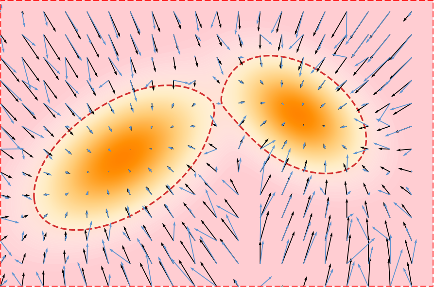
To address these challenges, Song and Ermon (2019) propose injecting Gaussian noise at multiple levels into the data distribution and jointly training a noise-conditional score network (NCSN) to estimate score functions across a range of noise scales. During generation, Langevin dynamics is applied in a noise-annealed fashion: beginning with high-noise levels to enable coarse exploration, and gradually refining toward low-noise levels to recover fine details.
Training
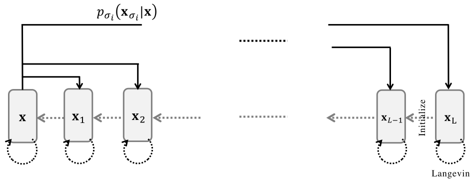
To overcome the limitations of score-based models trained at a single noise level, Song and Ermon (2019) propose adding Gaussian noise at multiple levels to the data distribution. Specifically, a sequence of \(L\) noise levels \(\{\sigma_i\}_{i=1}^L\) is chosen such that \[0 < \sigma_1 < \sigma_2 < \cdots < \sigma_L,\] where \(\sigma_1\) is small enough to preserve most of the data’s fine details, and \(\sigma_L\) is large enough to sufficiently smooth the distribution, facilitating easier training.
Each noisy sample is constructed by perturbing a clean data point \({\mathbf{x}}\sim p_{\text{data}}\) as \({\mathbf{x}}_{\sigma} = {\mathbf{x}}+ \sigma \bm{\epsilon}\) with \(\bm{\epsilon} \sim \mathcal{N}(\bm{0}, {\mathbf{I}})\). This defines the
Perturbation Kernel:
\[p_{\sigma}({\mathbf{x}}_{\sigma} | {\mathbf{x}}) := \mathcal{N}({\mathbf{x}}_{\sigma}; {\mathbf{x}}, \sigma^2 {\mathbf{I}}),\] which induces the
Marginal Distribution:
\[p_\sigma({\mathbf{x}}_{\sigma}) = \int p_{\sigma} ({\mathbf{x}}_{\sigma} | {\mathbf{x}}) p_{\text{data}}({\mathbf{x}}) \mathop{}\!\mathrm{d}{\mathbf{x}},\] at each noise level \(\sigma\). It presents the Gaussian smoothed data distribution.
Training Objective of NCSN.
The goal is to train a noise-conditional score network \({\mathbf{s}}_{\bm{\phi}}({\mathbf{x}}, \sigma)\) to estimate the score function \(\nabla_{{\mathbf{x}}} \log p_\sigma({\mathbf{x}})\) for all \(\sigma \in \{\sigma_i\}_{i=1}^L\). This is achieved by minimizing the DSM objective across all noise levels: \[\begin{align} \label{eq:nscn} \mathcal{L}_{\text{NCSN}}(\bm{\phi}) := \sum_{i=1}^{L} \lambda(\sigma_i) \mathcal{L}_{\text{DSM}}(\bm{\phi}; \sigma_i), \end{align}\] where \[\begin{align*} \mathcal{L}_{\text{DSM}}(\bm{\phi}; \sigma) = \frac{1}{2} \mathbb{E}_{{\mathbf{x}}\sim p_{\text{data}}({\mathbf{x}}), \tilde{{\mathbf{x}}} \sim p_{\sigma}(\tilde{{\mathbf{x}}} | {\mathbf{x}})} \left[ \left\lVert{\mathbf{s}}_{\bm{\phi}}(\tilde{{\mathbf{x}}}, \sigma) - \left( \frac{{\mathbf{x}}- \tilde{{\mathbf{x}}}}{\sigma^2} \right)\right\rVert_2^2 \right], \end{align*}\] and \(\lambda(\sigma_i)>0\) is a weighting function for each scale.
Minimizing this objective yields the score model \({\mathbf{s}}^*({\mathbf{x}}, \sigma)\) that recovers the true score at each noise level: \[{\mathbf{s}}^*(\cdot, \sigma) = \nabla_{{\mathbf{x}}} \log p_\sigma(\cdot), \quad \text{for all } \sigma \in \{\sigma_i\}_{i=1}^L,\] as it is essentially DSM minimization (see Theorem: Equivalence of L_SM and L_DSM).
Relationship with DDPM Loss.
Let \({\mathbf{x}}_\sigma={\mathbf{x}}+\sigma\boldsymbol{\epsilon}\) with \(\boldsymbol{\epsilon}\sim\mathcal{N}(\mathbf{0},\mathbf{I})\) and let \(p_\sigma\) denote the marginal distribution. By Tweedie’s formula, \[\nabla_{{\mathbf{x}}_\sigma}\log p_\sigma({\mathbf{x}}_\sigma) = -\frac{1}{\sigma} \mathbb{E}\left[\boldsymbol{\epsilon} \middle| {\mathbf{x}}_\sigma\right].\] Thus the NCSN optimum is the true score \({\mathbf{s}}^*({\mathbf{x}}_\sigma,\sigma)=\nabla_{{\mathbf{x}}_\sigma}\log p_\sigma({\mathbf{x}}_\sigma)\), while the Bayes optimal noise predictor under the DDPM loss Equation in Chapter 2 is \(\boldsymbol{\epsilon}^*({\mathbf{x}}_\sigma,\sigma)=\mathbb{E}[\boldsymbol{\epsilon}|{\mathbf{x}}_\sigma]\). They are exactly equivalent via \[{\mathbf{s}}^*({\mathbf{x}}_\sigma,\sigma) = - \frac{1}{\sigma} \boldsymbol{\epsilon}^*({\mathbf{x}}_\sigma,\sigma), \qquad \boldsymbol{\epsilon}^*({\mathbf{x}}_\sigma,\sigma) = - \sigma {\mathbf{s}}^*({\mathbf{x}}_\sigma,\sigma).\] In the DDPM setting, the noisy sample at step \(i\) can be written as \[\sigma_i:=\sqrt{1-\bar{\alpha}_i^2}, \qquad {\mathbf{x}}_i = \bar{\alpha}_i{\mathbf{x}}_0+\sigma_i{\bm{\epsilon}}, \qquad {\bm{\epsilon}}\sim\mathcal{N}(\bm{0},{\mathbf{I}}).\] Therefore, the score and the optimal noise prediction contain the same information: \[{\mathbf{s}}^*({\mathbf{x}}_i,i) = -\frac{1}{\sigma_i} \mathbb{E}\left[{\bm{\epsilon}}|{\mathbf{x}}_i\right].\] In other words, predicting the noise in DDPM is equivalent, up to the known scale factor \(1/\sigma_i\), to predicting the score at noise level \(i\).
We will systematically compare and summarize this equivalence of parameterizations in Chapter 6.
Sampling
Algorithm: Annealed Langevin Dynamics
Input: Trained score \({\mathbf{s}}_{\bm{\phi}^\times}(\cdot,\sigma_\ell)\), step sizes \(\eta_\ell\), and Langevin iteration budgets \(N_\ell\) for each noise level \(\ell=L,\ldots,1\); initialization distribution \(p_{\mathrm{init}}\)
\({\mathbf{x}}\sim p_{\mathrm{init}}\)
// Initialize from unstructured noise at the largest noise level
for \(\ell=L,L-1,\ldots,1\) do
\(\tilde{{\mathbf{x}}}_0 \gets {\mathbf{x}}\)
// Initialize this noise level from the previous level’s output
for \(n=0\) to \(N_\ell-1\) do
\(\bm{\epsilon}_n \sim \mathcal{N}(\bm{0},{\mathbf{I}})\)
\(\tilde{{\mathbf{x}}}_{n+1} \gets \tilde{{\mathbf{x}}}_n +\eta_\ell {\mathbf{s}}_{\bm{\phi}^\times}(\tilde{{\mathbf{x}}}_n,\sigma_\ell) +\sqrt{2\eta_\ell}\,\bm{\epsilon}_n\)
\({\mathbf{x}}\gets \tilde{{\mathbf{x}}}_{N_\ell}\)
// Pass the final state to the next smaller noise level, if any
Output: \({\mathbf{x}}\)
With trained score networks available at multiple noise levels \[{\mathbf{s}}_{\bm{\phi}^\times}(\cdot, \sigma_1), \quad{\mathbf{s}}_{\bm{\phi}^\times}(\cdot, \sigma_2), \quad \cdots, \quad {\mathbf{s}}_{\bm{\phi}^\times}(\cdot, \sigma_{L-1}), \quad {\mathbf{s}}_{\bm{\phi}^\times}(\cdot, \sigma_L),\]
the sampling procedure known as annealed Langevin dynamics (Song and Ermon 2019) generates data by progressively denoising from a high noise level \(\sigma_L\) down to a low noise level \(\sigma_1 \approx 0\).
With trained scores at noise levels \(0<\sigma_1<\cdots<\sigma_L\), annealed Langevin dynamics generates samples by moving gradually from high noise to low noise. Starting from a simple initialization \({\mathbf{x}}\sim p_{\mathrm{init}}\), it first applies Langevin dynamics at the largest noise level \(\sigma_L\), whose score \({\mathbf{s}}_{\bm{\phi}^\times}(\cdot,\sigma_L)\) guides the samples toward the corresponding smoothed distribution \(p_{\sigma_L}\). The resulting samples are then used to initialize Langevin dynamics at the next smaller noise level. Repeating this procedure progressively refines the samples until the smallest noise level \(\sigma_1\) is reached.
At each noise level \(\sigma_\ell\), Langevin dynamics performs the update \[\tilde{{\mathbf{x}}}_{n+1} = \tilde{{\mathbf{x}}}_n + \eta_\ell {\mathbf{s}}_{\bm{\phi}^\times}(\tilde{{\mathbf{x}}}_n,\sigma_\ell) + \sqrt{2\eta_\ell}\,\bm{\epsilon}_n, \qquad \bm{\epsilon}_n\sim\mathcal{N}(\bm{0},{\mathbf{I}}),\] where the output from the previous noise level provides the initialization \(\tilde{{\mathbf{x}}}_0\). A common choice is to scale the step size with the noise level as \[\eta_\ell = \delta\frac{\sigma_\ell^2}{\sigma_1^2}, \qquad \delta>0.\] The algorithm performs Langevin updates at every noise level, including \(\sigma_1\), so the final sample is obtained after refinement at the smallest noise level. Algorithm (Annealed Langevin Dynamics) summarizes the procedure.
The initial distribution \(p_{\mathrm{init}}\) simply provides a starting point for the Markov chain. At the largest noise level, Langevin dynamics moves this initial distribution toward \(p_{\sigma_L}\), after which the successive noise levels gradually guide the samples toward increasingly less smoothed versions of the data distribution.
Slow Sampling Speed of NCSN.
NCSN generates samples using annealed MCMC (commonly Langevin dynamics) across noise scales \(\{\sigma_i\}_{i=1}^L\). For each scale \(\sigma_i\), it performs \(K\) iterative updates of the form “update \(\tilde{\mathbf{x}}_n\) using the score \({\mathbf{s}}_{\bm{\phi}^\times}(\tilde{\mathbf{x}}_n,\sigma_i)\) plus a small random perturbation”, each requiring a forward pass through the score network. Two factors necessitate large \(L \times K\):
Local Accuracy and Stability: the learned score is reliable only for small perturbations, requiring small step sizes and many iterations per noise level to avoid bias or instability;
Slow Mixing in High Dimensions: local MCMC moves explore multimodal, high-dimensional targets inefficiently, demanding many iterations to reach typical data regions.
Because updates are strictly sequential (each iteration depends on the previous one) and each requires an expensive network evaluation, the overall cost is \(\mathcal{O}(L K)\) sequential network passes, making sampling computationally slow.
Summary: A Comparative View of NCSN and DDPM
We begin by comparing the graphical models of NCSN and DDPM in Figure 1.7, with key differences and similarities summarized in Table 1.1.
| NCSN | DDPM | ||
|---|---|---|---|
| \({\mathbf{x}}_{i+1}|{\mathbf{x}}_{i}\) | Derive as \({\mathbf{x}}_{i+1} = {\mathbf{x}}_i + \sqrt{\sigma^2_{i+1}-\sigma^2_{i}}\bm{\epsilon}\) | Define as \({\mathbf{x}}_{i+1} = \sqrt{1-\beta_{i}} {\mathbf{x}}_{i} + \sqrt{\beta_{i}}\bm{\epsilon}\) | |
| \({\mathbf{x}}_{i}|{\mathbf{x}}\) | Define as \({\mathbf{x}}_{i} = {\mathbf{x}}+ \sigma_{i}\bm{\epsilon}\) | Derive as \({\mathbf{x}}_i = \bar{\alpha}_i{\mathbf{x}}+ \sqrt{1 - \bar{\alpha}_i^2}\bm{\epsilon}\) | |
| \(p_{\text{prior}}\) | \(\mathcal{N}(\bm{0}, \sigma_L^2{\mathbf{I}})\) | \(\mathcal{N}(\bm{0}, {\mathbf{I}})\) | |
| Loss | \(\mathbb{E}_{i} \mathbb{E}_{p_{\text{data}}({\mathbf{x}})} \mathbb{E}_{\bm{\epsilon} \sim \mathcal{N}\left(\mathbf{0}, {\mathbf{I}}\right)} \left[ \left\lVert{\mathbf{s}}_{\bm{\phi}}({\mathbf{x}}_i, \sigma_i) + \frac{\bm{\epsilon}}{\sigma_i}\right\rVert_2^2 \right]\) | \(\mathbb{E}_{i}\mathbb{E}_{p_{\text{data}}({\mathbf{x}})} \mathbb{E}_{\bm{\epsilon}\sim \mathcal{N}(\bm{0},{\mathbf{I}})}\left[ \left\lVert\bm{\epsilon}_{\bm{\phi}}({\mathbf{x}}_i, i) - \bm{\epsilon}\right\rVert_2^2 \right]\) | |
| Sampling | Apply Langevin per layer; use output to initialize the next | Traversing the Markovian chain with \(p_{\bm{\phi}^\times}({\mathbf{x}}_{i-1} | {\mathbf{x}}_i)\) |
A Shared Bottleneck.
Despite their different formulations, both NCSN and DDPM rely on dense time discretization. This leads to a critical limitation: sampling often requires hundreds or even thousands of iterations, making generation slow and computationally intensive.
How can we accelerate sampling in diffusion models?
We return to this challenge in Chapter 9, which develops more efficient samplers; Chapter 10, which compresses pretrained diffusion models requiring hundreds of sampling steps into fewer-step student generators; and Chapter 11, which studies how to learn fast few-step generators directly from scratch under diffusion-inspired principles.
Closing Remarks
This chapter has charted a second major path to diffusion models, beginning from the score-based perspective rooted in Energy-Based Models (EBMs). We started by identifying the core challenge of EBMs—the intractable partition function—and introduced the score function, \(\nabla_{\mathbf{x}}\log{p(\mathbf{x})}\), as a powerful tool that circumvents this issue entirely.
Our journey led us from classic score matching to its more scalable and robust variant, Denoising Score Matching (DSM). Through DSM, we saw how perturbing data with noise enables a tractable training objective, once again leveraging a conditioning strategy to create a simple regression target. Furthermore, we established a profound connection between score estimation and the act of denoising via Tweedie’s formula, which showed that the score provides the precise direction needed to estimate a clean signal from its noisy observation.
This principle was then extended from a single noise level to a ladder of noise levels with Noise Conditional Score Networks (NCSN), which learn a single score model conditioned on multiple noise scales and generate samples via annealed Langevin dynamics. The next chapter takes the additional step from this discrete ladder to a continuum of noise levels through the Score SDE framework.
This convergence is no coincidence; it hints at a deeper, unified mathematical structure. The limitations of these discrete-time models motivate the need for a more general framework. In the next chapter, we will take this crucial step:
We will move into a continuous-time perspective, showing that both DDPMs and NCSNs can be elegantly unified as different discretizations of a single, powerful process described by a Stochastic Differential Equation (SDE).
This Score SDE framework will formally connect the variational and score-based views, recasting the problem of generation as one of solving a differential equation.
This unifying lens will not only provide profound theoretical clarity but also unlock a new class of advanced numerical methods designed to tackle the fundamental challenge of slow sampling.
With the factor \(\sqrt{2}\), the Langevin dynamics leave \(p_{\bm\phi}\) unchanged in time. Namely, \(p_{\bm\phi}\) is stationary: if \({\mathbf{x}}(0)\sim p_{\bm\phi}\) then \({\mathbf{x}}(t)\sim p_{\bm\phi}\) for all \(t\ge 0\). Equivalently, \(p_{\bm\phi}\) is the stationary solution of the Fokker–Planck equation (see Appendix B): \[\partial_t \rho = -\nabla \cdot(\rho \nabla\log p_{\bm\phi}) + \tfrac{\sigma^2}{2}\Delta \rho.\] Setting \(\rho=p_{\bm\phi}\) gives \((\tfrac{\sigma^2}{2}-1)\Delta p_{\bm\phi}=0\), which holds only if \(\sigma=\sqrt{2}\).↩︎
Brownian increments satisfy \(\mathbf{w}(t+\eta)-\mathbf{w}(t)\sim \mathcal{N}(\mathbf{0}, \eta \mathbf{I})\). Euler–Maruyama therefore uses a step noise \(\sqrt{2} [\mathbf{w}(t+\eta)-\mathbf{w}(t)] = \sqrt{2\eta} \bm{\epsilon}_n\) with \(\bm{\epsilon}_n \sim \mathcal{N}(\mathbf{0},\mathbf{I})\), which explains the \(\sqrt{\eta}\) factor.; this is the source of the square-root scaling. For a detailed introduction to Brownian motion and SDEs, please refer to Appendix A.↩︎
We remark that strict concavity (and thus a strict local maximum of the log density) requires the entire Hessian \(\nabla_{{\mathbf{x}}}^2 u\) to be negative definite, not merely to have negative trace. A negative trace guarantees that the sum of eigenvalues is negative, but some eigenvalues could still be positive, leading to a saddle point rather than a maximum.↩︎