Appendix B: Density Evolution: From Change of Variable to Fokker–Planck

Understanding how probability densities evolve under transformations is fundamental in both probability theory and generative modeling. In particular, diffusion models aim to construct generative processes whose induced density paths reverse a pre-defined forward process. This evolution is governed by the continuity equation or, in the stochastic case, the Fokker-Planck equation.

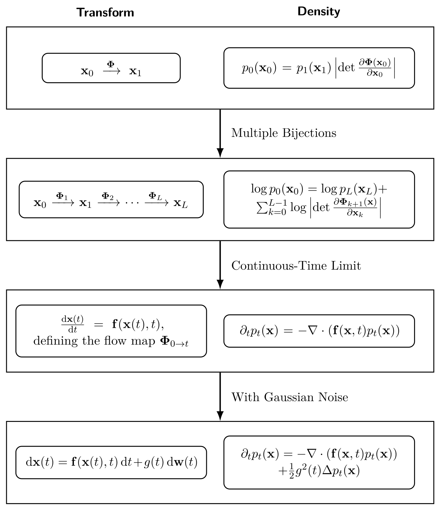
Although these names may sound unfamiliar or intimidating, they are in fact continuous-time analogues of the change-of-variable formula from basic calculus. In Section 1.1, it builds up to them by presenting a progression of change-of-variable formulas, starting from deterministic bijections, and culminating in stochastic differential equations. This progression naturally bridges discrete mappings and continuous-time flow dynamics. See Figure 1.1 for an overview of this unified framework.

In Section 1.2, we provide a physical and intuitive interpretation of the continuity equation, emphasizing its connection to the conservation of density in dynamical systems.

Change-of-Variable Formula:
From Deterministic Maps to Stochastic Flows

In this section, we aim to demystify the continuity equation and the Fokker-Planck equation by drawing analogies to the classic change-of-variable formula from calculus. We begin with the familiar single-variable case, extend it to the multivariate setting and to probability densities (Section 1.1.1), then generalize to compositions of bijective maps whose continuous-time limit leads to the continuity equation (Section 1.1.2). Finally, we incorporate stochasticity by introducing random noise, which naturally extends the continuity equation to the Fokker-Planck equation (Section 1.1.3).

Change-of-Variable Formula for Deterministic Maps

We move particles according to a deterministic map and study how their law (density) evolves. The key principle is conservation of probability mass, grounded in a fundamental result from calculus and probability: the change-of-variable formula. This formula describes how integrals, and therefore probability densities, transform under smooth bijective mappings. To build intuition, we first consider a single update step, and then extend the discussion to sequential transformations.

Single Update.

Think of a single update rule induced by applying a vector field (analogous to a force) \(\bm{\Psi}:\mathbb{R}^D \to \mathbb{R}^D\) for one unit of time. Starting from an initial particle state \({\mathbf{x}}_0\), its next state is given by \[{\mathbf{x}}_1 = \bm{\Psi}({\mathbf{x}}_0).\]

Underlying Pattern (a Density) and How it Moves.

If the initial states follow an underlying “law/pattern” described by a density \(p_0\) (i.e., \({\mathbf{x}}_0\sim p_0\)), then applying \(\bm{\Psi}\) produces a new density \(p_1\) for \({\mathbf{x}}_1\) (i.e., \({\mathbf{x}}_1\sim p_1\)). Assuming \(\bm{\Psi}\) is a smooth bijection, \(p_1\) is obtained from \(p_0\) via the standard change-of-variables formula:

Here \(\tfrac{\partial \bm{\Psi}}{\partial {\mathbf{x}}}\) is the Jacobian matrix of \(\bm{\Psi}\), denoted \(\partial_{\mathbf{x}}\bm{\Psi}\). Equivalently, in the original coordinates, \[p_0({\mathbf{x}}_0) \;=\; p_1\!\big(\bm{\Psi}({\mathbf{x}}_0)\big)\;\big|\det \partial_{\mathbf{x}}\bm{\Psi}({\mathbf{x}}_0)\big|.\] In words, \(\bm{\Psi}\) reshapes the density \(p_0\) into \(p_1\). The factor \(\big|\det \partial_{\mathbf{x}}\bm{\Psi}\big|\) represents the local change in volume; since probability mass is conserved, the density compensates by its inverse.

As a simple case, if \(\bm{\Psi}\) is linear with an invertible matrix \({\mathbf{A}}\) (i.e., \({\mathbf{x}}_1={\mathbf{A}}{\mathbf{x}}_0\)), then \[p_1({\mathbf{x}}_1)\;=\;p_0({\mathbf{A}}^{-1}{\mathbf{x}}_1)\,\big|\det {\mathbf{A}}^{-1}\big|.\]

Schematically, we can read it as: \[\begin{array}{lccc} \mathbf{Sample:} & {\mathbf{x}}_0 & \xrightarrow{\hspace{0.2cm} \bm{\Psi} \hspace{0.2cm}} & {\mathbf{x}}_1 \\ \mathbf{Density:} & p_{{\mathbf{x}}_0}({\mathbf{x}}_0) & \xrightarrow{\hspace{0.2cm} \bm{\Psi} \hspace{0.2cm}} & p_{{\mathbf{x}}_1}({\mathbf{x}}_1) \end{array}\]

Why is Equation \(\eqref{eq:change-of-variable-density}\) the Change-of-Variables Formula?

This comes directly from the familiar rule in calculus.

Single-Variable Case.

Let \(y = \Psi(x)\) be smooth and invertible. Rewriting an integral over \(y\) in terms of \(x\) gives \[\int g(y)\,\mathop{}\!\mathrm{d}y = \int g(\Psi(x)) \cdot |\Psi'(x)|\,\mathop{}\!\mathrm{d}x,\] where \(|\Psi'(x)|\) compensates for interval stretching or compression, ensuring area preservation.

Multivariate Case.

For \(\bm{\Psi}: \mathbb{R}^D \to \mathbb{R}^D\) with \({\mathbf{y}}=\bm{\Psi}({\mathbf{x}})\), \[\int g({\mathbf{y}})\,\mathop{}\!\mathrm{d}{\mathbf{y}} = \int g(\bm{\Psi}({\mathbf{x}})) \,\big|\det(\partial_{\mathbf{x}}\bm{\Psi})\big| \,\mathop{}\!\mathrm{d}{\mathbf{x}},\] so infinitesimal volumes transform as \[\mathop{}\!\mathrm{d}{\mathbf{y}}= \big|\det(\partial_{\mathbf{x}}\bm{\Psi})\big|\,\mathop{}\!\mathrm{d}{\mathbf{x}}.\]

From this, the density formula in Equation \(\eqref{eq:change-of-variable-density}\) follows: \[\begin{align*} p_{{\mathbf{y}}}({\mathbf{y}}) = \int_{\mathbb{R}^D} \delta({\mathbf{y}}- \bm{\Psi}({\mathbf{x}}))\, p_{{\mathbf{x}}}({\mathbf{x}})\mathop{}\!\mathrm{d}{\mathbf{x}}= p_{{\mathbf{x}}}\!\big(\bm{\Psi}^{-1}({\mathbf{y}})\big)\,\Big|\det\!\left(\frac{\partial \bm{\Psi}^{-1}}{\partial {\mathbf{y}}}\right)\Big|. \end{align*}\]

Composing Multiple Bijections.

We now apply several updates in sequence. Let \({\mathbf{x}}_k = \bm{\Psi}_k({\mathbf{x}}_{k-1})\) for \(k=1,\dots,L\); that is, \[{\mathbf{x}}_0 \xrightarrow{\ \bm{\Psi}_1\ } {\mathbf{x}}_1 \xrightarrow{\ \bm{\Psi}_2\ } \cdots \xrightarrow{\ \bm{\Psi}_L\ } {\mathbf{x}}_L,\] where each \(\bm{\Psi}_k:\mathbb{R}^D \to \mathbb{R}^D\) is a smooth bijection. If the initial state follows density \(p_0\) (i.e., \({\mathbf{x}}_0 \sim p_0\)), then the sequence of updates induces densities \(p_1,\dots,p_L\) for \({\mathbf{x}}_1,\dots,{\mathbf{x}}_L\).

Because probability mass is conserved at each step, the densities evolve according to \[p_{k}({\mathbf{x}}_k) \;=\; p_{k-1}({\mathbf{x}}_{k-1}) \, \Big|\det \partial_{{\mathbf{x}}_{k-1}} \bm{\Psi}_k({\mathbf{x}}_{k-1})\Big|^{-1}, \quad k=1,\dots,L.\] By recursion, the final density at \({\mathbf{x}}_L\) is

Equivalently, in log-density form: \[\begin{align*} \log p_{{\mathbf{x}}_L}({\mathbf{x}}_L) = \log p_{{\mathbf{x}}_0}({\mathbf{x}}_0) - \sum_{k=1}^L \log \left| \det \left( \frac{\partial \bm{\Psi}_k}{\partial {\mathbf{x}}_{k-1}} \right) \right|. \end{align*}\] This expression reflects how each transformation \(\bm{\Psi}_k\) stretches or contracts volume, as captured by the Jacobian determinant. The accumulation of these local volume changes along the transformation path determines the final probability density under the composed map.

Equation \(\eqref{eq:cov-multi-layer-nolog}\) serves as the core principle underlying Normalizing Flows (see Section (Neural ODEs) in Chapter 5).

Continuous-Time Limit: Continuity Equation

We now pass from discrete updates to a continuous description. Suppose the particle motion is driven by a time-varying velocity field \({\mathbf{f}}:\mathbb{R}^D \times [0,T]\to \mathbb{R}^D\). Imagine evolving a particle \({\mathbf{x}}_0 \sim p_0\) through infinitely many small bijective updates. At each step \(t\) of length \(\Delta t>0\), the update is \[{\mathbf{x}}_{t+\Delta t} = \bm{\Psi}({\mathbf{x}}_t) := {\mathbf{x}}_t + \Delta t\, {\mathbf{f}}({\mathbf{x}}_t, t).\] As \(\Delta t \to 0\), the composition of these updates converges to a continuous flow governed by a velocity field \({\mathbf{f}}:\mathbb{R}^D \times [0,T]\to \mathbb{R}^D\): \[\begin{align} \label{eq:ode-f-continuity} \frac{\mathop{}\!\mathrm{d}{\mathbf{x}}(t)}{\mathop{}\!\mathrm{d}t} = {\mathbf{f}}({\mathbf{x}}(t), t), \qquad {\mathbf{x}}(0) = {\mathbf{x}}_0 \sim p_0. \end{align}\] Under suitable smoothness assumptions (see Appendix A), this ODE admits a unique solution for each initial condition, which defines a deterministic flow map \(\bm{\Psi}_{0\to t}:\mathbb{R}^D \to \mathbb{R}^D\). In other words, \(\bm{\Psi}_{0\to t}\) brings the initial state \({\mathbf{x}}_0\) to the solution of Equation \(\eqref{eq:ode-f-continuity}\) at time \(t\): \[\bm{\Psi}_{0\to t}({\mathbf{x}}_0) = {\mathbf{x}}_0 + \int_{0}^{t} {\mathbf{f}}({\mathbf{x}}(\tau), \tau)\,\mathop{}\!\mathrm{d}\tau.\] As a result, the whole distribution also moves: the initial density \(p_0\) is transported into the new density \(p_t\), the law of \({\mathbf{x}}(t)\). Formally, this is written as a pushforward: \[p_t = \big(\bm{\Psi}_{0\to t}\big)_{\#} p_0.\] When \(\bm{\Psi}_{0\to t}\) is smooth and invertible, this reduces to the familiar change-of-variables rule: \[p_t({\mathbf{x}}) = p_0\!\big(\bm{\Psi}_{t\to 0}({\mathbf{x}})\big)\, \big|\det \partial_{\mathbf{x}}\bm{\Psi}_{t\to 0}({\mathbf{x}})\big| = \int \delta\!\left({\mathbf{x}}- \bm{\Psi}_{0\to t}({\mathbf{x}}_0)\right) p_0({\mathbf{x}}_0)\,\mathop{}\!\mathrm{d}{\mathbf{x}}_0.\]

Continuity Equation: How the Density Moves in Time.

Rather than writing a separate formula for the density at each time, we can describe how it moves continuously using a differential equation in space \({\mathbf{x}}\) and time \(t\). The idea is simple: probability mass is conserved, and the velocity field \({\mathbf{f}}\) only redistributes it in space. This gives the continuity equation:

Here the divergence term \(\nabla \cdot (p_t {\mathbf{f}})\) measures how the flow locally expands or compresses the density, ensuring total probability remains \(1\).

This partial differential equation (PDE) ensures that probability mass is conserved as the flow moves particles. In fact, it can be viewed as the continuous-time analogue of the change-of-variables formula.

Derivation of Continuity Equation via Change-of-Variables Formula.

Conceptually, the continuity equation can also be obtained by taking the continuous-time limit of Equation \(\eqref{eq:cov-multi-layer-nolog}\). Here, however, we adopt a more direct derivation based on Equation \(\eqref{eq:change-of-variable-density}\).

Discretization and Change-of-Variable Formula.

Consider \[\mathbf{x}_{t+\Delta t} := \bm{\Psi}(\mathbf{x}_t) = \mathbf{x}_t + \Delta t\, {\mathbf{f}}(\mathbf{x}_t, t),\] which is actually the forward Euler discretization of the ODE in Equation \(\eqref{eq:ode-f-continuity}\) over a small time interval \(\Delta t > 0\). The Jacobian of the map \(\bm{\Psi}\) with respect to \(\mathbf{x}_t\) expands as \[\frac{\partial \bm{\Psi}}{\partial \mathbf{x}_t} = {\mathbf{I}}+ \Delta t \nabla_{\mathbf{x}} {\mathbf{f}}(\mathbf{x}_t, t) + \mathcal{O}(\Delta t^2),\] so its determinant satisfies \[\det\left( \frac{\partial \bm{\Psi}}{\partial \mathbf{x}_t} \right) = 1 + \Delta t\, \nabla \cdot {\mathbf{f}}(\mathbf{x}_t, t) + \mathcal{O}(\Delta t^2).\] This uses the standard expansion \(\det({\mathbf{I}}+ \Delta t\, \mathbf{A}) = 1 + \Delta t\, \mathop{\mathrm{Tr}}(\mathbf{A}) + \mathcal{O}(\Delta t^2)\) as \(\Delta t \to 0\), along with \(\nabla \cdot {\mathbf{f}}= \mathop{\mathrm{Tr}}(\nabla_{\mathbf{x}} {\mathbf{f}})\).

Applying the change-of-variables formula, the log-density evolves as \[\begin{align*} \log p_{t+\Delta t}(\mathbf{x}_{t+\Delta t}) = \log p_t(\mathbf{x}_t) - \Delta t\, \nabla \cdot {\mathbf{f}}(\mathbf{x}_t, t) + \mathcal{O}(\Delta t^2). \end{align*}\] That is, \[\begin{align} \label{eq:log-density-diff} \log p_{t+\Delta t}(\mathbf{x}_{t+\Delta t}) - \log p_t(\mathbf{x}_t) = - \Delta t\, \nabla \cdot {\mathbf{f}}(\mathbf{x}_t, t) + \mathcal{O}(\Delta t^2). \end{align}\]

Using Taylor Expansion.

Now, we expand the left-hand side via multivariate Taylor expansion: \[\begin{align*} &\log p_{t+\Delta t}({\mathbf{x}}_{t+\Delta t}) - \log p_t({\mathbf{x}}_t) \\= &\Delta t\, \partial_t \log p_t({\mathbf{x}}_t) + ({\mathbf{x}}_{t+\Delta t} - {\mathbf{x}}_t)^\top \nabla_{{\mathbf{x}}_t} \log p_t({\mathbf{x}}_t) + \mathcal{O}(\Delta t^2). \end{align*}\] Substituting \({\mathbf{x}}_{t+\Delta t} - {\mathbf{x}}_t = {\mathbf{f}}({\mathbf{x}}_t, t)\Delta t\) yields: \[\begin{align*} &\log p_{t+\Delta t}({\mathbf{x}}_{t+\Delta t}) - \log p_t({\mathbf{x}}_t) \\= & \Delta t\, \partial_t \log p_t({\mathbf{x}}_t) + \Delta t\, {\mathbf{f}}({\mathbf{x}}_t, t)^\top \nabla_{{\mathbf{x}}_t} \log p_t({\mathbf{x}}_t) + \mathcal{O}(\Delta t^2). \end{align*}\] Matching terms with Equation \(\eqref{eq:log-density-diff}\) and letting \(\Delta t \to 0\), we conclude that \[\begin{equation*} \partial_t \log p_t({\mathbf{x}}_t) = - \nabla_{{\mathbf{x}}_t} \cdot {\mathbf{f}}({\mathbf{x}}_t, t) - {\mathbf{f}}({\mathbf{x}}_t, t)^\top \nabla_{{\mathbf{x}}_t} \log p_t({\mathbf{x}}_t). \end{equation*}\] Exponentiating and using the product rule yields the continuity equation.

Lagrangian and Eulerian Views of Deterministic Transport.

The same deterministic transport admits two complementary descriptions. The Lagrangian view follows individual particles through the flow map \(\bm{\Psi}_{0\to t}\), whereas the Eulerian view describes the velocity \({\mathbf{f}}({\mathbf{x}},t)\) and density \(p_t({\mathbf{x}})\) at fixed spatial locations. Under suitable regularity, these descriptions are consistent: a prescribed velocity field generates a particle flow, whose pushforward density satisfies the continuity equation.

There is nevertheless an important asymmetry. Once the velocity field and initial density are fixed, the resulting flow and density evolution are determined. A prescribed density path alone, however, generally does not determine a unique velocity field or particle flow.

From Velocity to Flow and Density.

So far, we have assumed that the velocity field \({\mathbf{f}}\) is given. The particle ODE \[\frac{\mathop{}\!\mathrm{d}{\mathbf{x}}(t)}{\mathop{}\!\mathrm{d}t} = {\mathbf{f}}({\mathbf{x}}(t), t)\] describes how each particle moves, while the density PDE \[\partial_t p_t + \nabla \!\cdot \!\big(p_t {\mathbf{f}}_t\big) = 0\] describes how the entire distribution of particles evolves. These two views are connected: moving particles according to the ODE automatically produces a density that satisfies the PDE. In this case, the particle flow \(\bm{\Psi}_{0\to t}\) is uniquely determined: starting from \({\mathbf{x}}(0)\sim p_0\), each trajectory \({\mathbf{x}}(t)\) is fixed, and the resulting density \(p_t\) follows the continuity equation. Here, particle dynamics and density dynamics are fully consistent.

From Density Path to Velocity: Non-Uniqueness.

If instead we begin only with the density path \(t \mapsto p_t\) (e.g., Section (Conditional Probability-Path-First Construction of v_t(·|z) and p_t(·|z)) in Chapter 5 in flow matching), the velocity field is no longer uniquely determined. For example, if a vector field \(\mathbf w_t\) satisfies \[\nabla_{{\mathbf{x}}}\cdot\!\big(p_t({\mathbf{x}})\,\mathbf w_t({\mathbf{x}})\big)=0 \qquad\text{(no net flux w.r.t.\ }p_t\text{),}\] then both \({\mathbf{f}}_t\) and \({\mathbf{f}}_t+\mathbf w_t\) give rise to the same density evolution. Thus a single density path may correspond to many different flows, and choosing one particular particle flow \(\bm{\Psi}_{0\to t}\) amounts to picking a specific velocity field among these possibilities.

Not every given path \(p_t\) can actually arise from particles moving under some velocity field. The continuity equation (Equation \(\eqref{eq:continuity-cov}\)) provides the consistency check for whether a density path can be “generated by a flow”. We say that \(p_t\) is realizable (or generated by \({\mathbf{f}}\)) if there exists a velocity field \({\mathbf{f}}\) such that particles following \[\dfrac{\mathop{}\!\mathrm{d}{\mathbf{x}}(t)}{\mathop{}\!\mathrm{d}t} = {\mathbf{f}}({\mathbf{x}}(t), t)\] produce exactly the densities \(p_t\) through the flow map \(\bm{\Psi}_{0\to t}\). That is, realizability holds when \(p_t\) and \({\mathbf{f}}\) together satisfy Equation \(\eqref{eq:continuity-cov}\).

Intuitively, realizability means that the snapshots of \(p_t\) over time can be explained by particles moving under some velocity field, rather than being an arbitrary sequence of distributions.

When this condition holds, the density \(p_t\) is nothing more than the pushforward of the initial density \(p_0\) along the flow map \(\bm{\Psi}_{0\to t}\). In this case, the familiar change-of-variables formula applies: \[\begin{align*} p_t = \big(\bm{\Psi}_{0\to t}\big)_{\#} p_0 = p_0\!\big(\bm{\Psi}_{t\to 0}({\mathbf{x}})\big)\, \big|\det \partial_{\mathbf{x}}\bm{\Psi}_{t\to 0}({\mathbf{x}})\big| = \int \delta \left({\mathbf{x}}- \bm{\Psi}_{0\to t}({\mathbf{x}}_0)\right) p_0({\mathbf{x}}_0)\,\mathop{}\!\mathrm{d}{\mathbf{x}}_0. \end{align*}\]

(Optional) Conditioning.

If an additional conditioning variable \({\mathbf{z}}\sim \pi({\mathbf{z}})\) is introduced, the same reasoning applies for each fixed \({\mathbf{z}}\): \[\frac{\mathop{}\!\mathrm{d}{\mathbf{x}}(t)}{\mathop{}\!\mathrm{d}t}={\mathbf{v}}_t({\mathbf{x}}(t)|{\mathbf{z}})\] with pushforward \(p_t(\cdot|{\mathbf{z}})=({\bm{\Psi}}_{0\to t}(\cdot;{\mathbf{z}}))_{\#}p_0\), and continuity equation \[\partial_t p_t({\mathbf{x}}|{\mathbf{z}})+\nabla\!\cdot\!\big(p_t({\mathbf{x}}|{\mathbf{z}})\,{\mathbf{v}}_t({\mathbf{x}}|{\mathbf{z}})\big)=0\] The marginal density is then \[p_t({\mathbf{x}})=\int p_t({\mathbf{x}}|{\mathbf{z}})\pi({\mathbf{z}})\mathop{}\!\mathrm{d}{\mathbf{z}}.\]

Stochastic Processes: Fokker-Planck Equation

When noise is added, the dynamics follow the SDE as in Equation in Appendix A \[\mathop{}\!\mathrm{d}{\mathbf{x}}(t) = {\mathbf{f}}({\mathbf{x}}(t), t)\mathop{}\!\mathrm{d}t + g(t)\mathop{}\!\mathrm{d}{\mathbf{w}}(t).\] Then, the density \(p_t({\mathbf{x}})\) satisfies the Fokker-Planck equation:

\(\Delta p_t = \nabla \cdot \nabla_{\mathbf{x}}p_t\) is the Laplacian operator. In the first equality, the first term describes transport of probability mass by the deterministic drift \({\mathbf{f}}\), while the second term models the spreading (diffusion) of the density due to stochastic noise with variance proportional to \(\tfrac{1}{2} g^2(t)\). The second equality rewrites the same density evolution as a continuity equation with velocity \[{\mathbf{f}}({\mathbf{x}},t) - \frac{1}{2}g^2(t)\nabla_{{\mathbf{x}}}\log p_t({\mathbf{x}}).\] Therefore, the deterministic ODE driven by this velocity therefore evolves through the same one-time marginal densities \(p_t\) as the SDE. This is the probability-flow ODE used throughout the book.

The derivation of the Fokker-Planck equation is more involved; we refer the reader to Section (Itô’s Formula’s Application: Derivation of Fokker-Planck Equation) in Appendix C.

Intuition of the Continuity Equation

In this section, we give a physical interpretation of the continuity equation, highlighting its role as a conservation law for probability density in a dynamical system.

Physical Interpretation of the Continuity Equation

Consider a small fixed control volume (a rectangular box) in 3D space with one corner at \(\mathbf{x} = (x, y, z)\) and side lengths \(\Delta x\), \(\Delta y\), and \(\Delta z\). Let \(p(\mathbf{x}, t)\) denote the density of a conserved quantity (e.g., mass or probability) at position \(\mathbf{x}\) and time \(t\). For a sufficiently small box, the total amount of the quantity inside the box is approximately: \[\text{Total quantity in box} \approx p(\mathbf{x}, t) \Delta x \Delta y \Delta z.\]

How Does the Total Change?

Changes in the total quantity can only arise from flux across the box’s boundary. Let \(\mathbf{j}(\mathbf{x}, t)\) denote the flux vector, representing the amount of quantity flowing per unit area per unit time.

Flux in the \(x\)-Direction.

The inflow through the left face (at \(x\)) is approximately: \[j_x(x, y, z, t) \Delta y \Delta z,\] and the outflow through the right face (at \(x + \Delta x\)) is: \[j_x(x + \Delta x, y, z, t) \Delta y \Delta z.\] Thus, the net influx in the \(x\)-direction is: \[\left[ j_x(x, y, z, t) - j_x(x + \Delta x, y, z, t) \right] \Delta y \Delta z.\]

Net Flux in All Directions.

Analogous terms arise in the \(y\)- and \(z\)-directions: \[\begin{align*} \left[ j_y(x, y, z, t) - j_y(x, y + \Delta y, z, t) \right] \Delta x \Delta z, \\ \left[ j_z(x, y, z, t) - j_z(x, y, z + \Delta z, t) \right] \Delta x \Delta y. \end{align*}\] Summing all contributions, the total net influx into the box is: \[- \nabla \cdot \mathbf{j}(\mathbf{x}, t) \Delta x \Delta y \Delta z.\] Equivalently, the total net outflux from the box is: \[\nabla \cdot \mathbf{j}(\mathbf{x}, t) \Delta x \Delta y \Delta z.\]

Rate of Change Inside the Box.

The rate of change of the total quantity within the box is: \[\frac{\partial p}{\partial t}(\mathbf{x}, t) \Delta x \Delta y \Delta z.\]

Conservation Principle.

Assuming the quantity is conserved (e.g., total mass or probability is constant in time), the rate of change equals the negative of the net outflux: \[\frac{\partial p}{\partial t}(\mathbf{x}, t) \Delta x \Delta y \Delta z = - \nabla \cdot \mathbf{j}(\mathbf{x}, t) \Delta x \Delta y \Delta z.\]

Canceling the common volume factor and taking the small-box limit, we obtain the local form of the continuity equation: \[\frac{\partial p}{\partial t} + \nabla \cdot \mathbf{j} = 0.\] This equation has a simple interpretation: if \(\nabla\cdot\mathbf{j}(\mathbf{x},t)>0\), more quantity flows out of the small box than into it, so the density inside decreases. If \(\nabla\cdot\mathbf{j}(\mathbf{x},t)<0\), more quantity flows in than out, so the density inside increases.

Derivation of the Continuity Equation from Conservation Laws

The small-box argument above gives the local intuition. We now write the same conservation principle in a coordinate-free form over an arbitrary control volume.

The continuity equation formalizes the conservation of a physical quantity, such as mass or charge, in a dynamical system. Let \(p(\mathbf{x}, t)\) denote the density of the conserved quantity at position \(\mathbf{x} \in \mathbb{R}^D\) and time \(t \in [0, T]\), and let \(\mathbf{v}(\mathbf{x}, t)\) denote the velocity field. When the quantity is transported by particles moving with velocity \(\mathbf{v}(\mathbf{x},t)\), the flux is \[\mathbf{j}(\mathbf{x},t)=p(\mathbf{x},t)\mathbf{v}(\mathbf{x},t).\]

Step 1: Rate of Change within a Control Volume.

Consider an arbitrary control volume \(V \subset \mathbb{R}^D\) with boundary \(\partial V\). The total amount of the conserved quantity in \(V\) is \[\int_V p(\mathbf{x}, t) \mathop{}\!\mathrm{d}V,\] whose time derivative gives the rate of accumulation: \[\frac{\partial}{\partial t} \int_V p(\mathbf{x}, t) \mathop{}\!\mathrm{d}V.\]

Step 2: Net Flux Through the Boundary.

The quantity exits \(V\) through \(\partial V\) with outward normal vector \(\mathbf{n}\). The net outward flux is \[\int_{\partial V} p(\mathbf{x}, t) \mathbf{v}(\mathbf{x}, t) \cdot \mathbf{n} \mathop{}\!\mathrm{d}S.\]

Step 3: Conservation Principle.

Conservation implies that the rate of accumulation within \(V\) equals the negative of the net outward flux: \[\frac{\partial}{\partial t} \int_V p \mathop{}\!\mathrm{d}V + \int_{\partial V} p \mathbf{v} \cdot \mathbf{n} \mathop{}\!\mathrm{d}S = 0.\]

Step 4: Divergence Theorem.

Applying the divergence theorem to convert the surface integral to a volume integral: \[\int_{\partial V} p \mathbf{v} \cdot \mathbf{n} \mathop{}\!\mathrm{d}S = \int_V \nabla \cdot (p \mathbf{v}) \mathop{}\!\mathrm{d}V.\] Hence, \[\frac{\partial}{\partial t} \int_V p \mathop{}\!\mathrm{d}V + \int_V \nabla \cdot (p \mathbf{v}) \mathop{}\!\mathrm{d}V = 0.\] Equivalently, \[\int_V \left(\frac{\partial p}{\partial t}+\nabla\cdot(p\mathbf{v})\right)\mathop{}\!\mathrm{d}V=0.\] Since the control volume \(V\) is arbitrary, the integrand must vanish pointwise. This yields the continuity equation: \[\frac{\partial p}{\partial t}+\nabla\cdot(p\mathbf{v})=0.\] Using \(\mathbf{j}=p\mathbf{v}\), this is the same as \[\frac{\partial p}{\partial t}+\nabla\cdot\mathbf{j}=0.\]

Particle-Level Intuition.

Expanding the divergence term gives \[\frac{\partial p}{\partial t} + \mathbf{v}\cdot\nabla p + p\,\nabla\cdot\mathbf{v} = 0.\] The first two terms describe the total change of the density along a moving particle: \[\frac{\mathop{}\!\mathrm{d}}{\mathop{}\!\mathrm{d}t}p(\mathbf{x}_t,t) = \frac{\partial p}{\partial t}(\mathbf{x}_t,t) + \mathbf{v}(\mathbf{x}_t,t)\cdot\nabla p(\mathbf{x}_t,t).\] Therefore, \[\frac{\mathop{}\!\mathrm{d}}{\mathop{}\!\mathrm{d}t}p(\mathbf{x}_t,t) = - p(\mathbf{x}_t,t)\nabla\cdot\mathbf{v}(\mathbf{x}_t,t).\] This provides another useful interpretation: density decreases when nearby particles spread apart, and density increases when nearby particles contract. Thus, the velocity field tells us how individual particles move, while the continuity equation tells us how the entire density evolves.

(Optional) Wasserstein Gradient Flows as Distribution-Level Training

We now step back from diffusion-specific dynamics and take a broader distribution-level view of deep generative modeling. We have discussed that the continuity equation describes how a probability distribution moves when its particles move. The same language can also be used to understand the training of deep generative models: a training algorithm updates the model parameters, the updated generator moves generated particles, and the movement of these particles changes the induced model distribution \(p_{{\bm{\phi}}}\).

From this viewpoint, different generative modeling methods can be organized according to how the model distribution \(p_{{\bm{\phi}}}\) is driven toward the data distribution \(p_{\mathrm{data}}\). Wasserstein gradient flow gives one particularly clean way to describe this movement: it treats training as an idealized flow of probability mass in distribution space, which is then approximated by finite-dimensional neural network updates.

A neural generator \({\mathbf{G}}_{{\bm{\phi}}}\) defines both a function and a probability distribution. If \[{\mathbf{z}}\sim p_{\mathrm{prior}}, \qquad {\mathbf{x}}={\mathbf{G}}_{{\bm{\phi}}}({\mathbf{z}}),\] then the generated distribution is the pushforward \[p_{{\bm{\phi}}}:=({\mathbf{G}}_{{\bm{\phi}}})_\# p_{\mathrm{prior}}.\] From the generative modeling viewpoint, the object we ultimately care about is how \(p_{{\bm{\phi}}}\) approaches the data distribution \(p_{\mathrm{data}}\).

This motivates a distribution-level question:

Throughout this optional section, \(\tau\) denotes training time: an idealized continuous-time version of the discrete training iteration index. It should not be confused with diffusion/noising time. We write \({\bm{\phi}}_\tau\) for the parameter at training time \(\tau\), and \(p_{{\bm{\phi}}_\tau}\) for the corresponding model distribution.

Moving Model Distributions by Moving Particles.

We first describe an ideal distribution-level evolution, before accounting for the finite-dimensional parameterization of the neural generator. Suppose particles from the current model distribution move according to a training-time velocity field \({\mathbf{w}}_\tau\): \[\frac{\mathop{}\!\mathrm{d}{\mathbf{x}}_\tau}{\mathop{}\!\mathrm{d}\tau} = {\mathbf{w}}_\tau({\mathbf{x}}_\tau), \qquad {\mathbf{x}}_\tau\sim p_{{\bm{\phi}}_\tau}.\] Then the model distribution evolves according to the continuity equation \[\partial_\tau p_{{\bm{\phi}}_\tau}({\mathbf{x}}) + \nabla_{{\mathbf{x}}}\cdot \big( p_{{\bm{\phi}}_\tau}({\mathbf{x}}){\mathbf{w}}_\tau({\mathbf{x}}) \big) = 0.\] Thus, \({\mathbf{w}}_\tau\) describes how each generated particle moves, while the continuity equation describes how the entire generated distribution moves¹.

Choosing the Velocity: Gradient Descent in Distribution Space.

Now we need to choose a velocity field \({\mathbf{w}}_\tau\) that moves \(p_{{\bm{\phi}}_\tau}\) toward \(p_{\mathrm{data}}\). Let \[\mathcal{D}(p_{{\bm{\phi}}_\tau},p_{\mathrm{data}})\] be a discrepancy between the current model distribution and the data distribution. Wasserstein gradient flow (Jordan et al. 1998; Ambrosio et al. 2005) chooses the particle velocity that decreases this discrepancy most directly under the geometry of moving probability mass.

To choose the velocity field, we first ask how the discrepancy changes when the current distribution is infinitesimally perturbed. Think of \(\mathcal{D}(p,p_{\mathrm{data}})\) as a global energy of the distribution \(p\). Its first variation gives a pointwise energy potential: it tells us which regions of space are costly for the current distribution and which regions are favorable.

Concretely, for a small perturbation \(p+\epsilon h\), where \(\epsilon>0\) is small and \(\int h({\mathbf{x}})\mathop{}\!\mathrm{d}{\mathbf{x}}=0\), the first variation is defined by \[\mathcal{D}(p+\epsilon h,p_{\mathrm{data}}) = \mathcal{D}(p,p_{\mathrm{data}}) + \epsilon \int \frac{\delta\mathcal{D}}{\delta p} (p,p_{\mathrm{data}})({\mathbf{x}})\, h({\mathbf{x}})\mathop{}\!\mathrm{d}{\mathbf{x}} + \mathop{\mathrm{o}}(\epsilon).\] Here \(p\) is a dummy distribution variable. After taking the variation, we evaluate it at the current model distribution \(p=p_{{\bm{\phi}}_\tau}\).

We define the resulting pointwise energy potential by \[E_\tau({\mathbf{x}}) := \frac{\delta\mathcal{D}}{\delta p} (p_{{\bm{\phi}}_\tau},p_{\mathrm{data}})({\mathbf{x}}).\] Intuitively, if \(E_\tau({\mathbf{x}})\) is large, then placing more probability mass near \({\mathbf{x}}\) would increase the discrepancy. If \(E_\tau({\mathbf{x}})\) is small, then moving mass toward \({\mathbf{x}}\) is favorable. Therefore, the Wasserstein gradient-flow velocity moves particles downhill in this potential: \[{\mathbf{w}}_\tau({\mathbf{x}}) = - \nabla_{{\mathbf{x}}}E_\tau({\mathbf{x}}).\] With this choice, \[\frac{\mathop{}\!\mathrm{d}}{\mathop{}\!\mathrm{d}\tau} \mathcal{D}(p_{{\bm{\phi}}_\tau},p_{\mathrm{data}}) = - \int p_{{\bm{\phi}}_\tau}({\mathbf{x}}) \left\| \nabla_{{\mathbf{x}}}E_\tau({\mathbf{x}}) \right\|_2^2 \mathop{}\!\mathrm{d}{\mathbf{x}} \le 0.\] Therefore, Wasserstein gradient flow is gradient descent in the \(2\)-Wasserstein geometry of probability distributions². The global discrepancy \(\mathcal{D}\) defines the energy of the whole distribution, the first variation \(E_\tau\) defines the local energy landscape seen by particles, and \(-\nabla_{{\mathbf{x}}}E_\tau\) gives the ideal particle velocity for decreasing the discrepancy.

Realizing the Distributional Velocity with a Neural Network.

The velocity above is a distribution-level object: it says how generated particles should move. A neural generator, however, cannot move every particle independently. It can only move particles through a shared parameter update of \({\bm{\phi}}\).

At training time \(\tau\), the current generator produces particles \[{\mathbf{x}}_i = {\mathbf{G}}_{{\bm{\phi}}_\tau}({\mathbf{z}}_i), \qquad {\mathbf{z}}_i\sim p_{\mathrm{prior}}, \qquad i=1,\ldots,N.\] A small Wasserstein step moves these particles to \[\widetilde{{\mathbf{x}}}_i = {\mathbf{x}}_i+\eta{\mathbf{w}}_\tau({\mathbf{x}}_i),\] where \(\eta>0\) is a small step size. The neural network is then updated so that its new outputs match these moved particles: \[{\bm{\phi}}_{\tau+\eta} \approx \arg\min_{{\bm{\phi}}} \frac{1}{N} \sum_{i=1}^N \left\| {\mathbf{G}}_{{\bm{\phi}}}({\mathbf{z}}_i) - \operatorname{sg} \big( {\mathbf{x}}_i+\eta{\mathbf{w}}_\tau({\mathbf{x}}_i) \big) \right\|_2^2.\] Here \(\operatorname{sg}(\cdot)\) denotes stop-gradient, so the moved particles are treated as fixed targets.

For a small parameter update \(\Delta{\bm{\phi}}\), we have the linearization \[{\mathbf{G}}_{{\bm{\phi}}_\tau+\Delta{\bm{\phi}}}({\mathbf{z}}_i) \approx {\mathbf{G}}_{{\bm{\phi}}_\tau}({\mathbf{z}}_i) + \big(\partial_{{\bm{\phi}}}{\mathbf{G}}_{{\bm{\phi}}_\tau}({\mathbf{z}}_i)\big)\Delta{\bm{\phi}}.\] Therefore, the parameter update approximately solves \[\min_{\Delta{\bm{\phi}}} \frac{1}{N} \sum_{i=1}^N \left\| \big(\partial_{{\bm{\phi}}}{\mathbf{G}}_{{\bm{\phi}}_\tau}({\mathbf{z}}_i)\big)\Delta{\bm{\phi}} - \eta{\mathbf{w}}_\tau({\mathbf{x}}_i) \right\|_2^2.\] In words, Wasserstein gradient flow specifies the desired distribution-level particle motion, while neural network training projects this motion onto the set of movements that can be realized by changing the finite-dimensional parameter \({\bm{\phi}}\).

Forward-KL Training: Data-Side Likelihood Learning.

A classical distribution-level objective is the data-side, or forward, KL divergence: \[\mathcal{D}_{\mathrm{FKL}}(p_{{\bm{\phi}}},p_{\mathrm{data}}) := \mathcal D_{\mathrm{KL}}(p_{\mathrm{data}}\|p_{{\bm{\phi}}}) = \int p_{\mathrm{data}}({\mathbf{x}}) \log \frac{p_{\mathrm{data}}({\mathbf{x}})}{p_{{\bm{\phi}}}({\mathbf{x}})} \mathop{}\!\mathrm{d}{\mathbf{x}}.\] Since \(p_{\mathrm{data}}\) is fixed, minimizing this objective is equivalent to maximum likelihood (see Equation in Chapter 1): \[\min_{{\bm{\phi}}} \mathcal D_{\mathrm{KL}}(p_{\mathrm{data}}\|p_{{\bm{\phi}}}) \quad \Longleftrightarrow \quad \max_{{\bm{\phi}}} \mathbb{E}_{{\mathbf{x}}\sim p_{\mathrm{data}}} \big[ \log p_{{\bm{\phi}}}({\mathbf{x}}) \big].\] This is the distribution-level view behind many likelihood-based models. Autoregressive models and normalizing flows optimize exact likelihoods; likelihood-based VAEs optimize variational lower bounds; energy-based models optimize likelihood through positive and negative phases; and diffusion models can be related to likelihood or score-matching surrogates through their variational and denoising objectives.

From the Wasserstein gradient-flow viewpoint, the forward KL has first variation \[\frac{\delta}{\delta p} \mathcal D_{\mathrm{KL}}(p_{\mathrm{data}}\|p) = - \frac{p_{\mathrm{data}}}{p}.\] Evaluating at \(p=p_{{\bm{\phi}}_\tau}\) gives the velocity \[{\mathbf{w}}_\tau^{\mathrm{FKL}}({\mathbf{x}}) = \nabla_{{\mathbf{x}}} \left( \frac{p_{\mathrm{data}}({\mathbf{x}})} {p_{{\bm{\phi}}_\tau}({\mathbf{x}})} \right).\] This expression involves the density ratio \(p_{\mathrm{data}}/p_{{\bm{\phi}}_\tau}\), which is usually difficult to estimate for implicit generators. In practice, forward-KL or maximum-likelihood training is most direct when likelihoods, variational bounds, or suitable approximations to the likelihood gradient are available. Score matching provides a different route to distribution learning by matching score functions rather than directly realizing the forward-KL Wasserstein flow.

The main strength of forward-KL training is that it is data-covering and statistically well grounded when a likelihood or a variational surrogate is available. Its limitation is that it often requires tractable densities, variational bounds, score-matching surrogates, or expensive negative sampling, which makes it less directly compatible with arbitrary implicit generators.

Reverse-KL Training: Model-Side Score-Mismatch Dynamics.

The model-side, or reverse, KL divergence is \[\mathcal{D}_{\mathrm{RKL}}(p_{{\bm{\phi}}},p_{\mathrm{data}}) := \mathcal D_{\mathrm{KL}}(p_{{\bm{\phi}}}\|p_{\mathrm{data}}) = \int p_{{\bm{\phi}}}({\mathbf{x}}) \log \frac{p_{{\bm{\phi}}}({\mathbf{x}})} {p_{\mathrm{data}}({\mathbf{x}})} \mathop{}\!\mathrm{d}{\mathbf{x}}.\] Its first variation is \[\frac{\delta}{\delta p} \mathcal D_{\mathrm{KL}}(p\|p_{\mathrm{data}}) = \log p-\log p_{\mathrm{data}}+1.\] Evaluating at \(p=p_{{\bm{\phi}}_\tau}\) gives the Wasserstein velocity \[{\mathbf{w}}_\tau^{\mathrm{RKL}}({\mathbf{x}}) := \nabla_{{\mathbf{x}}}\log p_{\mathrm{data}}({\mathbf{x}}) - \nabla_{{\mathbf{x}}}\log p_{{\bm{\phi}}_\tau}({\mathbf{x}}).\] Thus, reverse-KL training induces a score-mismatch force: \[\text{target score} - \text{model score}.\] The target score attracts generated particles toward high-density regions of the data distribution, while the model score repels particles from regions where the current model distribution is already too concentrated.

In diffusion distillation and distribution matching (see Section (Distribution-Based DistillationDistribution-Based Distillation) in Chapter 10), this idea is usually applied at a noise level \(s\). Let \(p_s\) denote the teacher or noised-data distribution, and let \(p_{{\bm{\phi}}_\tau,s}\) denote the noised distribution of current generator samples. The reverse-KL objective \[\mathbb{E}_s \left[ w(s) \mathcal D_{\mathrm{KL}}(p_{{\bm{\phi}}_\tau,s}\|p_s) \right]\] induces the score-mismatch velocity \[{\mathbf{w}}_{\tau,s}^{\mathrm{RKL}}({\mathbf{x}}) := \nabla_{{\mathbf{x}}}\log p_s({\mathbf{x}}) - \nabla_{{\mathbf{x}}}\log p_{{\bm{\phi}}_\tau,s}({\mathbf{x}}).\] At the parameter level, for generated noisy samples \(\hat{\mathbf{x}}_s\sim p_{{\bm{\phi}}_\tau,s}\), one obtains gradients of the form \[\nabla_{{\bm{\phi}}} \mathcal D_{\mathrm{KL}}(p_{{\bm{\phi}},s}\|p_s) \big|_{{\bm{\phi}}={\bm{\phi}}_\tau} = \mathbb{E}_{\hat{\mathbf{x}}_s\sim p_{{\bm{\phi}}_\tau,s}} \left[ \left( \nabla_{{\mathbf{x}}}\log p_{{\bm{\phi}}_\tau,s}(\hat{\mathbf{x}}_s) - \nabla_{{\mathbf{x}}}\log p_s(\hat{\mathbf{x}}_s) \right)^\top \partial_{{\bm{\phi}}}\hat{\mathbf{x}}_s \right].\] Thus, the score difference \[\nabla_{{\mathbf{x}}}\log p_s(\hat{\mathbf{x}}_s) - \nabla_{{\mathbf{x}}}\log p_{{\bm{\phi}}_\tau,s}(\hat{\mathbf{x}}_s)\] provides the distribution-level descent direction that drives the parameter gradient. The actual movement of individual generated samples is mediated by the shared neural parameterization, as discussed above. This score-difference gradient is the basic distribution-level mechanism behind reverse-KL-based methods such as DMD and VSD: estimate the target and model scores on generated samples and use their difference to update the generator.

The main strength of reverse-KL training is that it is naturally compatible with implicit generators once the relevant scores can be estimated. It is also mode-seeking, which can improve visual fidelity in one-step or few-step generation. Its limitation is that it can drop modes, depends strongly on the quality of score estimates, and may require an additional model-score network or a strong teacher.

The same attraction-repulsion interpretation also appears in drifting-style particle updates (Weber 2023; Deng et al. 2026). In the terminology of Lai et al. (2026), DMD/VSD/SiD provide parametric score-based instantiations of this score-mismatch dynamics, while drifting-style approaches (Weber 2023; Deng et al. 2026) provide a nonparametric kernel-based instantiation.

Closing Remarks.

In summary, the continuity equation provides the common language behind both diffusion dynamics and distribution-level training. In diffusion models, it describes how the intermediate distributions \(p_t\) evolve along a prescribed noise or probability-flow dynamics. In Wasserstein gradient flow, the same equation describes how the model distribution \(p_{{\bm{\phi}}_\tau}\) evolves during training as generated particles move toward the data distribution \(p_{\mathrm{data}}\).

This viewpoint therefore broadens the role of the continuity equation beyond diffusion models. It lets us interpret generative modeling as the design of distributional dynamics: different methods choose different discrepancies, different particle velocities, and different parameter updates to drive \(p_{{\bm{\phi}}}\) toward \(p_{\mathrm{data}}\). From this perspective, diffusion models, likelihood-based models, distribution-matching methods, and score-mismatch-based approaches can be viewed under a shared distribution-level taxonomy.