Chapter 11: Learning Fast Generators from Scratch
Truth is ever to be found in simplicity, and not in the multiplicity and confusion of things.
Isaac Newton
In Chapter 10, we saw that slow iterative samplers in diffusion models can be compressed into few-step generators through distillation. From an engineering perspective, two-stage pipelines are practical because they divide a complex generative training task into clear, independent objectives. The first stage learns the data distribution, while the second accelerates sampling or enhances quality. This separation allows each stage to be optimized independently, making the overall system easier to manage, more stable, and more reliable.
In this chapter, however, the focus shifts to a central question driving the progress of deep generative modeling:
Can we design a standalone generative principle that trains in a stable and efficient way, fast sampling, and allows users to easily guide or control what is produced?
In this chapter we pursue this direction and discuss an alternative approach: training few-step diffusion-based generators without relying on a pre-trained model. Our focus is the flow-map model. Here, a flow map is the classical solution map of an ODE, a notion rooted in differential equations and dynamical systems and closely connected, in continuum and fluid mechanics, to following the motion of material particles. Specifically, \({\bm{\Psi}}_{s\to t}\) takes a state at time \(s\) to the state reached at time \(t\) under the prescribed dynamics. A flow-map model learns to approximate this map directly, allowing a long trajectory to be traversed in one or a few network evaluations 1.
This formulation provides a principled way to transport probability mass from the prior distribution \(p_{\mathrm{prior}}\) to the data distribution \(p_{\mathrm{data}}\), while preserving the marginal distributions \(p_t\) specified by the forward diffusion process at each intermediate time.
After this chapter, you will be able to...
distinguish an instantaneous velocity field from its ODE solution map (flow map);
understand the semigroup property of exact ODE flows and how it motivates consistency-based learning objectives;
understand Consistency Model, Consistency Trajectory Model, and Mean Flow as representative ways to learn special or general flow maps;
distinguish oracle flow-map identities from their practical approximations, and understand how suitable parametrizations enable few-step generation while retaining access to local velocity information.
Reader route. The central object in this chapter is the ODE flow map. The individual methods should be viewed as different parametrizations and training strategies for learning this same underlying object.
Prologue

Motivation of Flow Map Models.
In Chapter 10 we showed how the inaccessible regression target in the oracle flow-map loss \(\mathcal{L}_{\mathrm{oracle}}({\bm{\theta}})\) (see Equation \(\eqref{eq:general-cm-loss:rep}\)) can be estimated by distilling knowledge from a pre-trained diffusion model to obtain few-step generators. This route is effective and practical: a two-stage pipeline can be engineered for robustness and often remains competitive in both data and compute efficiency.
In this chapter, we shift focus to a broader challenge at the core of deep generative modeling: Can we establish a standalone generative principle that enables stable, scalable, and efficient training, fast sampling, and generation that can be easily steered by user intentions, without relying on a pre-trained model? Designing such standalone principles lies at the center of generative modeling.
Diffusion models offer a useful design principle: start with a continuous-time forward process that gradually transforms data into a simple prior (noise) as a reference, and frame the modeling task as learning the reverse-time transport that restores this process to match the desired marginal distributions. This time-dependent formulation also makes it easier to steer the generation process at intermediate steps, compared to one-shot generative maps. Specializing to diffusion-motivated methods, this leads to the question:
Can we learn the flow map \({\bm{\Psi}}_{s\to t}(\cdot)\) with a network \({\mathbf{G}}_{\bm{\theta}}(\cdot,s,t)\) (a flow map model) without access to pre-trained models, while maintaining high-fidelity generation?
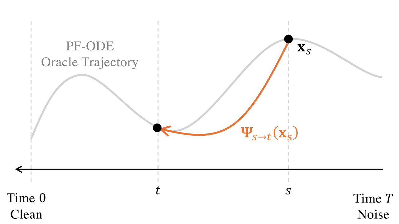
This chapter develops methods toward this goal, organized around a single objective that also underlies distillation and provides a unified view of flow-map formulations (Boffi et al. 2025; Hu et al. 2025):
\[\begin{equation} \label{eq:general-cm-loss:rep} \mathcal{L}_{\mathrm{oracle}}({\bm{\theta}}) := \mathbb{E}_{s,t}\,\mathbb{E}_{{\mathbf{x}}_s \sim p_s}\Big[ w(s,t) d\big({\mathbf{G}}_{\bm{\theta}}({\mathbf{x}}_s,s,t), {\bm{\Psi}}_{s\to t}({\mathbf{x}}_s)\big) \Big]. \end{equation}\]
Here \(s,t\) are sampled from some time distribution (e.g., uniform), \(w(s,t) \ge 0\) assigns weights to the time pairs \((s,t)\), and \(d(\cdot,\cdot)\) is a discrepancy measure such as the squared \(\ell_2\) norm. The oracle flow map \({\bm{\Psi}}_{s\to t}\) represents the ideal transformation that takes a state \({\mathbf{x}}_s\) at time \(s\) and transports it directly to time \(t\): \[{\bm{\Psi}}_{s\to t}({\mathbf{x}}_s) = {\mathbf{x}}_s + \int_s^t {\mathbf{v}}^*({\mathbf{x}}_u,u)\,\mathrm{d}u,\] where the oracle drift is given as \[{\mathbf{v}}^*({\mathbf{x}}_u,u) = \mathbb{E}\left[\alpha_u'{\mathbf{x}}_0+ \sigma_u'{\bm{\epsilon}}| {\mathbf{x}}_u\right],\] while equivalent parametrizations are also possible (see Chapter 6), with common choices including the \({\mathbf{x}}\)-prediction and \({\mathbf{v}}\)-prediction forms.
At the optimum of the oracle loss, the learned model recovers the true flow map exactly: \[{\mathbf{G}}^*({\mathbf{x}}_s, s, t) = {\bm{\Psi}}_{s\to t}({\mathbf{x}}_s), \quad \text{for all }\, s,t, \text{ and }\, {\mathbf{x}}_s \sim p_s.\]
Because the flow map \({\bm{\Psi}}_{s\to t}\) cannot be expressed in closed form, it must be approximated. One option, discussed in Chapter 10, is to rely on a pre-trained diffusion model. Alternatively, as we will see in this chapter, new and more tractable surrogates can be introduced. For clarity, existing approaches can be broadly categorized according to whether the training procedure queries a teacher during the loop: distillation, which explicitly calls a teacher model, and training from scratch, which avoids teacher calls by constructing self-contained surrogates.
Building on this principled objective, we now turn to systematic approaches for learning flow map models, with the aim of developing methods that are practical while also producing generations that more accurately reflect the true data distribution and are computationally efficient. We begin with a high-level introduction to this paradigm.
Special Flow Map: Consistency Functions.
Consistency Models (Song et al. 2023) represent one of the earliest pioneering approaches to flow-map learning. They learn a few-step denoiser \({\mathbf{f}}_{\bm{\theta}}(\cdot,s)\) that approximates the special case of the flow map to the origin: \[{\bm{\Psi}}_{s\to 0}(\cdot), \qquad s \in (0,T].\] The key idea is that every state \({\mathbf{x}}_s\) is mapped to the time-\(0\) endpoint \({\bm{\Psi}}_{s\to 0}({\mathbf{x}}_s)\) of the PF-ODE trajectory passing through it. Formally, the oracle training objective for the CM family (Song et al. 2023; Song and Dhariwal 2024; Geng et al. 2024; Lu and Song 2024) is \[\begin{align} \label{eq:oracle-cm} \mathcal{L}_{\mathrm{oracle}\text{-}\mathrm{CM}}({\bm{\theta}}) := \mathbb{E}_{s} \mathbb{E}_{{\mathbf{x}}_s\sim p_s} \left[ w(s) d \left({\mathbf{f}}_{\bm{\theta}}({\mathbf{x}}_s,s), {\bm{\Psi}}_{s\to 0}({\mathbf{x}}_s)\right)\right]. \end{align}\]
In practice, however, the oracle \({\bm{\Psi}}_{s\to 0}({\mathbf{x}}_s)\) is unavailable. It is therefore replaced by a stop-gradient target, denoted as \({\mathbf{f}}_{{\bm{\theta}}^-}\), taken from a slightly earlier step \({\bm{\Psi}}_{s\to s-\Delta s}({\mathbf{x}}_s)\) on the same trajectory: \[{\bm{\Psi}}_{s\to 0}({\mathbf{x}}_s) \approx {\mathbf{f}}_{{\bm{\theta}}^-} \left({\bm{\Psi}}_{s\to s-\Delta s}({\mathbf{x}}_s),\,s-\Delta s\right), \quad \Delta s > 0,\] where \({\bm{\Psi}}_{s\to s-\Delta s}({\mathbf{x}}_s)\) itself must also be approximated. Two practical strategies are available: (i) distillation, which relies on a pre-trained diffusion model, and (ii) training from scratch, which uses a one-point estimate without teacher guidance.
General Flow Map.
Two representative approaches are the Consistency Trajectory Model (CTM) and Mean Flow (MF).
Consistency Trajectory Models.
Consistency Trajectory Model (CTM)
(Kim, Lai, Liao,
Murata, et al. 2024) is the first work to learn the general flow
map \({\bm{\Psi}}_{s\to t}\) for
arbitrary start and end times, and can be viewed as a concrete instance
under the unified objective of Equation \(\eqref{eq:general-cm-loss:rep}\). CTM
adopts an Euler-inspired parametrization by expressing the oracle flow
map as \[\begin{align*}
{\bm{\Psi}}_{s\to t}({\mathbf{x}}_s)
:= {\mathbf{x}}_s + \int_s^t
{\mathbf{v}}^*({\mathbf{x}}_u,u)\mathop{}\!\mathrm{d}u
= \frac{t}{s} {\mathbf{x}}_s
+ \frac{s-t}{s}
\underbrace{\Big[{\mathbf{x}}_s + \frac{s}{s-t} \int_s^t
{\mathbf{v}}^*({\mathbf{x}}_u,u)
\mathop{}\!\mathrm{d}u\Big]}_{\approx~{\mathbf{g}}_{{\bm{\theta}}}},
\end{align*}\] which motivates the neural parameterization \[{\mathbf{G}}_{{\bm{\theta}}}({\mathbf{x}}_s,s,t)
:= \frac{t}{s}\,{\mathbf{x}}_s +
\frac{s-t}{s}\,{\mathbf{g}}_{\bm{\theta}}({\mathbf{x}}_s,s,t),\]
where \({\mathbf{g}}_{\bm{\theta}}\) is
a neural network trained so that \({\bm{\Psi}}_{s\to t}({\mathbf{x}}_s)\approx
{\mathbf{G}}_{{\bm{\theta}}}({\mathbf{x}}_s,s,t)\).
Since the oracle \({\bm{\Psi}}_{s\to t}({\mathbf{x}}_s)\) is inaccessible, CTM trains against a stop-gradient target evaluated at an intermediate time \(u\): \[{\bm{\Psi}}_{s\to t}({\mathbf{x}}_s) \approx {\mathbf{G}}_{{\bm{\theta}}^-} \big({\bm{\Psi}}_{s\to u}({\mathbf{x}}_s),\,u,\,t\big), \qquad u\in[t,s],\] where the intermediate state \({\bm{\Psi}}_{s\to u}({\mathbf{x}}_s)\) is approximated in one of two ways: (i) distillation, which uses a few-step solver applied to a pre-trained diffusion teacher, or (ii) training from scratch, which constructs a self-induced teacher directly through the \({\mathbf{G}}_{\bm{\theta}}\) parametrization.
Mean Flow.
Mean Flow (MF) (Geng, Deng, et al. 2025) builds on flow matching by modeling the average drift over an interval \([t,s]\) (with \(t\le s\)): \[{\mathbf{h}}_{{\bm{\theta}}}({\mathbf{x}}_s,s,t) \approx {\mathbf{h}}^*({\mathbf{x}}_s,s,t) := \frac{1}{\,t-s\,}\int_s^t {\mathbf{v}}^*({\mathbf{x}}_u,u)\,\mathop{}\!\mathrm{d}u,\] also aligning with Equation \(\eqref{eq:general-cm-loss:rep}\). Differentiating the identity \[(t-s)\,{\mathbf{h}}^*({\mathbf{x}}_s,s,t) = \int_s^t {\mathbf{v}}^*({\mathbf{x}}_u,u)\,\mathop{}\!\mathrm{d}u\] with respect to \(s\) yields a self-referential relation that motivates the MF objective \[\mathcal{L}_{\mathrm{MF}}({\bm{\theta}}) := \mathbb{E}_s\,\mathbb{E}_{{\mathbf{x}}_s\sim p_s} \Big[w(s)\,\big\| {\mathbf{h}}_{{\bm{\theta}}}({\mathbf{x}}_s,s,t)-{\mathbf{h}}_{{\bm{\theta}}^-}^{\mathrm{tgt}}({\mathbf{x}}_s,s,t) \big\|_2^2\Big],\] with stop-gradient target \[{\mathbf{h}}_{{\bm{\theta}}^-}^{\mathrm{tgt}}({\mathbf{x}}_s,s,t) := {\mathbf{v}}^*({\mathbf{x}}_s,s) - (s-t) \left((\partial_{\mathbf{x}}{\mathbf{h}}_{{\bm{\theta}}^-})\,{\mathbf{v}}^*({\mathbf{x}}_s,s) + \partial_s {\mathbf{h}}_{{\bm{\theta}}^-}\right).\] In practice, the oracle velocity \({\mathbf{v}}^*({\mathbf{x}}_s,s)\) must also be approximated. Two common strategies are: (i) distillation, which leverages a pre-trained diffusion model trained with flow matching, or (ii) training from scratch, which uses the one-point conditional velocity \(\alpha'_s\,{\mathbf{x}}_0+\sigma'_s\,{\bm{\epsilon}}\) derived from the forward corruption process \({\mathbf{x}}_s = \alpha_s {\mathbf{x}}_0+\sigma_s {\bm{\epsilon}}\).
Relationship Between CTM and MF.
CTM and MF approximate the same path integral but parameterize different surrogates of it: \[\begin{align*} {\bm{\Psi}}_{s\to t}({\mathbf{x}}_s) &:= {\mathbf{x}}_s + \int_s^t {\mathbf{v}}^*({\mathbf{x}}_u,u)\,\mathop{}\!\mathrm{d}u \\[2pt] &= \frac{t}{s}\,{\mathbf{x}}_s + \frac{s-t}{s}\, \underbrace{\Big[{\mathbf{x}}_s + \frac{s}{\,s-t\,} \int_s^t {\mathbf{v}}^*({\mathbf{x}}_u,u)\,\mathop{}\!\mathrm{d}u\Big]}_{\approx~{\mathbf{g}}_{{\bm{\theta}}} } \\[4pt] &= {\mathbf{x}}_s + (t-s)\, \underbrace{\Big[\frac{1}{\,t-s\,} \int_s^t {\mathbf{v}}^*({\mathbf{x}}_u,u)\,\mathop{}\!\mathrm{d}u\Big]}_{\approx~{\mathbf{h}}_{{\bm{\theta}}} }. \end{align*}\] In words, CTM learns an slope displacement through \({\mathbf{g}}_{\bm{\theta}}\), while MF learns the average drift \({\mathbf{h}}_{\bm{\theta}}\); both are consistent ways to approximate the same integral that defines \({\bm{\Psi}}_{s\to t}\).
What Happens Next?
We begin with the CM family, which focuses on the specific flow map \({\bm{\Psi}}_{s\to 0}\). This part covers both its discrete time origin in Section 1.2 and its continuous time extension in Section 1.3. We then move on to the general flow map and provide a detailed discussion of two key representatives, CTM and MF. Their parameterizations, training strategies, and practical approximations are presented in Section 1.4 and Section 1.5, respectively.
We remark that the Elucidating Diffusion Model (EDM) introduced in Section ((Optional) Elucidating Diffusion Model (EDM)) in Appendix D offers systematic guidelines for designing the network parameterization of the \({\mathbf{x}}\)-prediction model and has demonstrated strong empirical performance. Although this section can be considered optional, the EDM formulation serves as a valuable foundation for CM-style models.
For clarity of exposition later on, we do not strictly follow the chronological order in which these approaches appeared. Instead, we organize the discussion by conceptual relationships. Nevertheless, to acknowledge originality and respect chronology, we provide the historical timeline in Figure 1.1.
Special Flow Map: Consistency Model in Discrete Time
An Important Principle of Flow Maps: The Semigroup Property.
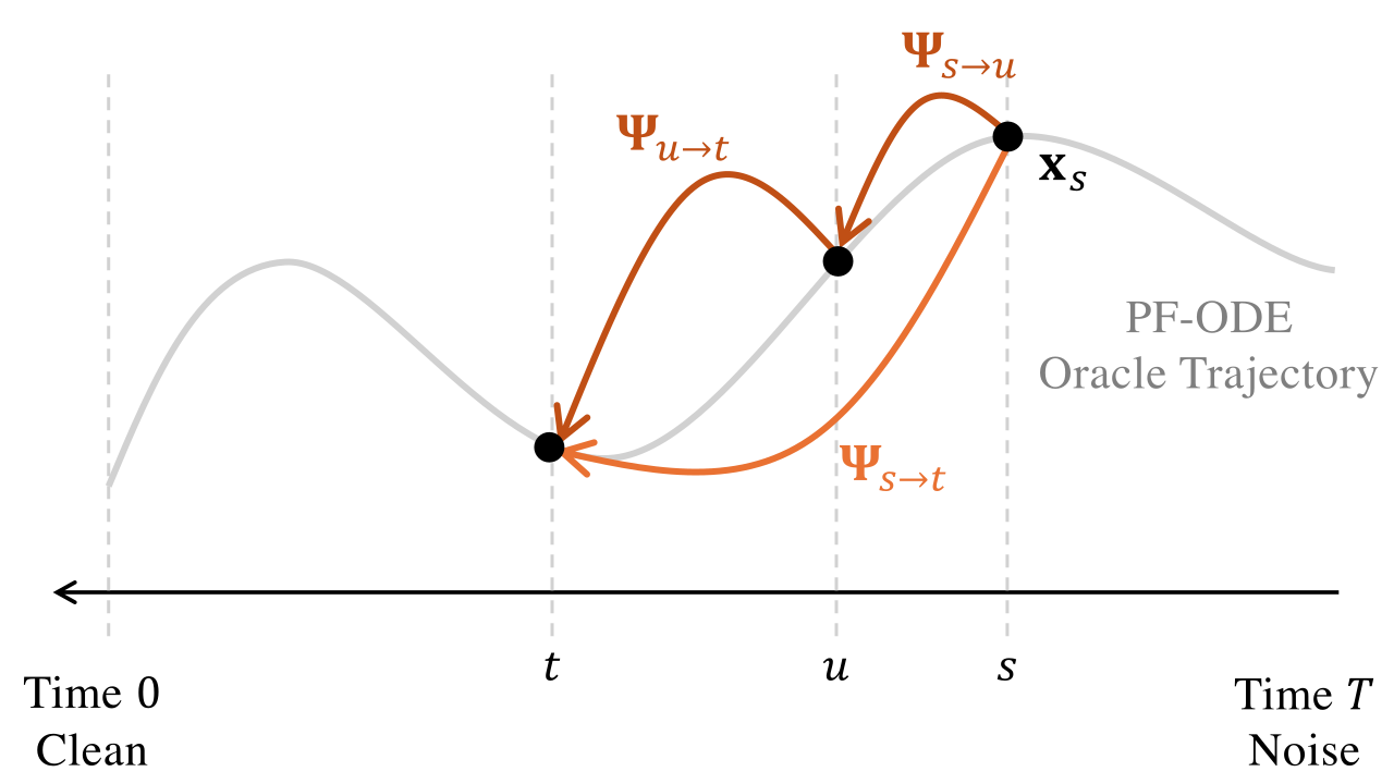
Consistency Models (introduced in Section (Special Flow Map: Consistency Model in Discrete Time) and Section (Special Flow Map: Consistency Model in Continuous Time)) and their generalization, the Consistency Trajectory Model (Section 1.4), define their regression targets by exploiting a key mathematical structure of flow maps. This structure is the fundamental semigroup property:
\[\begin{align} \label{eq:semi-group} {\bm{\Psi}}_{u\to t}\circ {\bm{\Psi}}_{s\to u}={\bm{\Psi}}_{s\to t}, \,\,\, {\bm{\Psi}}_{s\to s}={\mathbf{I}}, \quad \text{for all }\, s, u, t \in [0,T]. \end{align}\]
Intuitively, this means that if we first evolve a state from \(s\) to \(u\) (through \({\bm{\Psi}}_{s\rightarrow u}\)) and then from \(u\) to \(t\) (through \({\bm{\Psi}}_{u\rightarrow t}\)), we end up at exactly the same point as if we had evolved directly from \(s\) to \(t\). This is nothing more than the basic principle of ODE solving2: once the starting point of a flow is specified, its future evolution is completely determined, and it follows a single well-defined path. Whether we follow this path in one long step or divide it into smaller intervals, we still move along the same trajectory and arrive at the same final state.
To build further intuition for the semigroup property, consider the solution trajectory \(\{{\mathbf{x}}(s)\}_{s \in [0,T]}\) of the PF-ODE \[\begin{align*} \frac{\mathop{}\!\mathrm{d}{\mathbf{x}}(\tau)}{\mathop{}\!\mathrm{d}\tau} = {\mathbf{v}}^*({\mathbf{x}}(\tau), \tau), \end{align*}\] with a fixed initial condition \({\mathbf{x}}(T)\) at time \(T\), solved backward in time. If we fix the terminal time at \(t=0\), the corresponding flow map can be written more simply as \[{\mathbf{f}}^*(\cdot, s) := {\bm{\Psi}}_{s\to 0}(\cdot),\] which is referred to as the consistency function. By construction, this function inherits several fundamental properties directly from the semigroup identity of Equation \(\eqref{eq:semi-group}\) with \(t=0\):
Global Consistency: every point along the trajectory maps to the same clean endpoint, \[{\mathbf{f}}^*({\mathbf{x}}(s), s) = {\mathbf{x}}(0), \quad \text{for all }\, s \in [0,T].\] This is because \[\begin{align*} {\mathbf{f}}^*({\mathbf{x}}(s),s) &= {\bm{\Psi}}_{s\to 0}\big({\bm{\Psi}}_{0\to s}({\mathbf{x}}(0))\big) = \big({\bm{\Psi}}_{s\to 0}\circ {\bm{\Psi}}_{0\to s}\big)({\mathbf{x}}(0)) \\&= {\bm{\Psi}}_{0\to 0}({\mathbf{x}}(0)) = {\mathbf{x}}(0). \end{align*}\]
Self Consistency: any two points along the same trajectory must give identical outputs, \[\begin{align} \label{eq:cm-self-consistency} {\mathbf{f}}^*({\mathbf{x}}(s), s) = {\mathbf{f}}^*({\mathbf{x}}(u), u), \quad \text{for all }\, s, u \in [0,T]. \end{align}\] This is a direct re-interpretation of the semigroup identity: \(\Psi_{s\rightarrow 0}\circ\Psi_{0\rightarrow s}=\Psi_{u\rightarrow 0}\circ\Psi_{0\rightarrow u}\).
Local Consistency: the consistency function is invariant with respect to \(s\) when evaluated along the trajectory, \[\begin{align} \label{eq:cm-diff} \frac{\mathop{}\!\mathrm{d}}{\mathop{}\!\mathrm{d}s}\,{\mathbf{f}}^*({\mathbf{x}}(s),s) = 0, \qquad {\mathbf{f}}^*({\mathbf{x}}(0),0) = {\mathbf{x}}(0). \end{align}\] This follows from global consistency, which states that \({\mathbf{f}}^*({\mathbf{x}}(s), s)\) does not change with \(s\) along the trajectory.
The three properties are all equivalent. Each states that along any solution trajectory \(s\mapsto {\mathbf{x}}(s)\), the flow-to-origin/consistency map \({\mathbf{f}}^*({\mathbf{x}}(s),s)={\bm{\Psi}}_{s\to 0}({\mathbf{x}}(s))\) yields the same terminal point \({\mathbf{x}}(0)\), independent of the starting time.
Goal of Consistency Models.
A CM aims to train a neural network \({\mathbf{f}}_{\bm{\theta}} \colon \mathbb{R}^D \times [0,T] \to \mathbb{R}^D\) to approximate the special flow map \({\bm{\Psi}}_{s\to 0}\), i.e., consistency function3. The key idea is to enforce consistency along PF-ODE trajectories: states lying on the same ODE trajectory should map to the same time-\(0\) endpoint (more precisely, this corresponds to the special case \(t=0\) and \(u=s-\Delta s\) in Equation \(\eqref{eq:semi-group}\)).
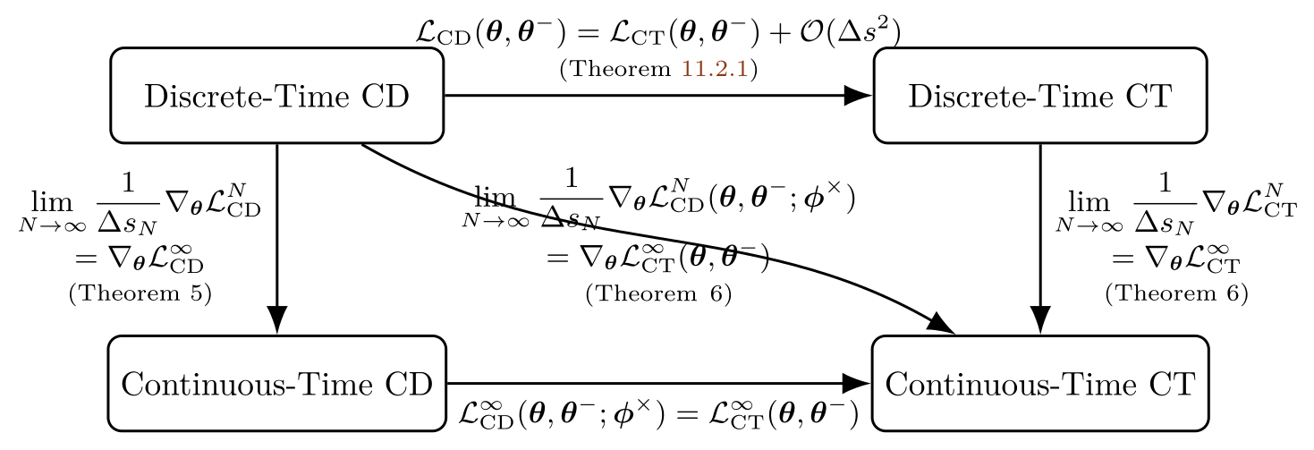
There are, however, multiple ways to realize this goal. The choice depends on whether a pre-trained diffusion model is available and whether training is carried out in a discrete-time or continuous-time regime. We begin by summarizing these variants in Table 1.1 and illustrating their objectives in Figure 1.4. The subsequent sections (Section (Special Flow Map: Consistency Model in Discrete Time) and Section (Special Flow Map: Consistency Model in Continuous Time)) then gradually develop the details of each approach.
| Distillation | From Scratch | |
|---|---|---|
| Discrete-time | Equation \(\eqref{eq:cd-discrete-approx-N}\) | Equation \(\eqref{eq:ct-discrete-approx-N}\) |
| Continuous-time | Equation \(\eqref{eq:cd-continuous-time}\) | Equation \(\eqref{eq:ct-continuous-time}\) |
Discrete-Time Approximations for Learning a Consistency Function
In principle, a consistency function can be learned by minimizing the oracle loss Equation \(\eqref{eq:oracle-cm}\): \[\mathcal{L}_{\mathrm{oracle}\text{-}\mathrm{CM}}({\bm{\theta}}) := \mathbb{E}_{s} \mathbb{E}_{{\mathbf{x}}_s\sim p_s} \left[ w(s) d \left({\mathbf{f}}_{\bm{\theta}}({\mathbf{x}}_s,s), {\bm{\Psi}}_{s\to 0}({\mathbf{x}}_s)\right)\right].\] This objective enforces that every noisy sample \({\mathbf{x}}_s\) is mapped back to its clean endpoint \({\bm{\Psi}}_{s\to 0}({\mathbf{x}}_s)\).
The challenge is that the oracle map \({\bm{\Psi}}_{s\to 0}({\mathbf{x}}_s)\) is not available in practice. To overcome this, Song et al. (2023) exploit the semigroup property: any noisy state and its consecutive step along the same PF-ODE trajectory must map to the same clean endpoint. Concretely, the oracle target is replaced by a stop-gradient target taken from a slightly earlier point on the trajectory: \[\begin{align*} {\bm{\Psi}}_{s\to 0}({\mathbf{x}}_s) &= {\bm{\Psi}}_{s-\Delta s \to 0} \left({\bm{\Psi}}_{s\to s-\Delta s}({\mathbf{x}}_s)\right) \\ &\approx {\mathbf{f}}_{{\bm{\theta}}^-} \left({\bm{\Psi}}_{s\to s-\Delta s}({\mathbf{x}}_s),\,s-\Delta s\right), \qquad \Delta s > 0, \end{align*}\] where \(\bm{\theta}^-\) are parameters under the stop-gradient operator. A further difficulty is that the intermediate state \({\bm{\Psi}}_{s\to s-\Delta s}({\mathbf{x}}_s)\) has no closed form either and must itself be approximated. Two practical regimes have been proposed:
With Pre-trained Diffusion Model (Consistency Distillation).
Suppose we have access to a pre-trained diffusion model. Consistency Distillation (CD) leverages the teacher model to approximate the intermediate state \({\bm{\Psi}}_{s\to s-\Delta s}({\mathbf{x}}_s)\) by simulating only a single backward ODE step: \[{\bm{\Psi}}_{s\to s-\Delta s}({\mathbf{x}}_s) \approx \mathtt{Solver}_{s \to s-\Delta s}({\mathbf{x}}_s).\]
More concretely, a pre-trained diffusion model provides an estimate of the score function \({\mathbf{s}}_{\bm{\phi}^\times}({\mathbf{x}}_s, s) \approx \nabla_{{\mathbf{x}}_s}\log p_s({\mathbf{x}}_s)\). Using this, one can perform a one-step DDIM update from \({\mathbf{x}}_s\) to obtain an approximation of the state at \(s' = s-\Delta s\): \[\begin{align*} {\bm{\Psi}}_{s\to s-\Delta s}({\mathbf{x}}_s) &\approx \frac{\alpha_{s'}}{\alpha_s}\,{\mathbf{x}}_s + \sigma_s^2 \left( \frac{\alpha_{s'}}{\alpha_s} - \frac{\sigma_{s'}}{\sigma_s} \right)\nabla_{{\mathbf{x}}_s}\log p_s({\mathbf{x}}_s) \\ &\approx \frac{\alpha_{s'}}{\alpha_s}\,{\mathbf{x}}_s + \sigma_s^2 \left( \frac{\alpha_{s'}}{\alpha_s} - \frac{\sigma_{s'}}{\sigma_s} \right){\mathbf{s}}_{\bm{\phi}^\times}({\mathbf{x}}_s, s) \\ &:= \tilde{{\mathbf{x}}}_{s'}^{\bm{\phi}^\times}. \end{align*}\]
Combining this construction with the stop-gradient target yields a practical discrete-time proxy for the oracle loss \(\mathcal{L}_{\mathrm{oracle}\text{-}\mathrm{CM}}({\bm{\theta}})\). Formally, over a partition \(0 = s_1 < s_2 < \cdots < s_N = T\), the CD training objective is given by
\[\begin{align} \label{eq:cd-discrete-approx-N} \mathcal{L}_{\text{CD}}^N(\bm{\theta}, \bm{\theta}^-; \bm{\phi}^\times) := \mathbb{E}_{{\mathbf{x}}_0, {\bm{\epsilon}}, i} \Big[\, \omega(s_i)\, d\big({\mathbf{f}}_{\bm{\theta}}({\mathbf{x}}_{s_{i+1}}, s_{i+1}),\, {\mathbf{f}}_{\bm{\theta}^-}(\tilde{{\mathbf{x}}}_{s_i}^{\bm{\phi}^\times}, s_i)\big)\Big]. \end{align}\]
Here, \(\omega(\cdot)\) is a time-dependent weight, \(d(\cdot,\cdot)\) is a distance measurement, and \(\bm{\theta}^-\) indicates stop-gradient parameters, which prevent collapse to trivial solutions (e.g., constant predictions).
Without Pre-Trained Diffusion Model (Consistency Training).
When no pre-trained diffusion model is available, the oracle score \(\nabla_{{\mathbf{x}}}\log p_s({\mathbf{x}}_s)\) can still be estimated directly using a simple one-point approximation (albeit with high variance). Recall that it admits the conditional expectation form: \[\begin{align*} \nabla_{{\mathbf{x}}_s} \log p_s({\mathbf{x}}_s) &= \mathbb{E}_{{\mathbf{x}}_0 \sim p({\mathbf{x}}_0|{\mathbf{x}}_s)} \left[ \nabla_{{\mathbf{x}}_s}\log p({\mathbf{x}}_s|{\mathbf{x}}_0) \right] \\ &= \mathbb{E}_{{\mathbf{x}}_0 \sim p({\mathbf{x}}_0|{\mathbf{x}}_s)} \left[ -\frac{{\mathbf{x}}_s - \alpha_s {\mathbf{x}}_0}{\sigma_s^2} \right]. \end{align*}\] The identity above suggests a simple one-sample estimator. If \({\mathbf{x}}_s\) is obtained from a paired sample \(({\mathbf{x}}_0,{\bm{\epsilon}})\) via \({\mathbf{x}}_s = \alpha_s {\mathbf{x}}_0 + \sigma_s {\bm{\epsilon}}\), then \[\widehat{\nabla_{{\mathbf{x}}}\log p_s}({\mathbf{x}}_s) :=-\frac{\boldsymbol\epsilon}{\sigma_s} =-\frac{{\mathbf{x}}_s-\alpha_s {\mathbf{x}}_0}{\sigma_s^2}\] serves as an unbiased estimator of the score at \({\mathbf{x}}_s\) (conditionally unbiased with respect to \(p({\mathbf{x}}_0|{\mathbf{x}}_s)\)). It corresponds exactly to the conditional score used as the regression target in denoising score matching.
Plugging this estimate into the DDIM one-step update from \(s\) to \(s' = s-\Delta s\) (see Equation in Chapter 9) yields \[\begin{align} \label{eq:one-pt-score} \begin{aligned} {\bm{\Psi}}_{s\to s'}({\mathbf{x}}_s) &\approx \frac{\alpha_{s'}}{\alpha_s}\,{\mathbf{x}}_s + \sigma_s^2 \left(\frac{\alpha_{s'}}{\alpha_s}-\frac{\sigma_{s'}}{\sigma_s}\right)\nabla_{{\mathbf{x}}_s}\log p_s({\mathbf{x}}_s) && \text{(DDIM)} \\ &\approx \frac{\alpha_{s'}}{\alpha_s}\,{\mathbf{x}}_s + \sigma_s^2 \left(\frac{\alpha_{s'}}{\alpha_s}-\frac{\sigma_{s'}}{\sigma_s}\right)\widehat{\nabla_{{\mathbf{x}}_s}\log p_s}({\mathbf{x}}_s) && \text{(1-pt score)} \\ &= \frac{\alpha_{s'}}{\alpha_s}\,{\mathbf{x}}_s -\left(\frac{\alpha_{s'}}{\alpha_s}-\frac{\sigma_{s'}}{\sigma_s}\right)({\mathbf{x}}_s-\alpha_s{\mathbf{x}}_0) \\ &= \alpha_{s'}{\mathbf{x}}_0+\sigma_{s'}{\bm{\epsilon}}, \end{aligned} \end{align}\] where4 \({\mathbf{x}}_0\) is the same data sample and \({\bm{\epsilon}}\) is the same Gaussian noise used to construct \({\mathbf{x}}_s\).
This leads to a teacher-free discrete-time surrogate of the oracle objective \(\mathcal{L}_{\mathrm{oracle}\text{-}\mathrm{CM}}\), written as
\[\begin{align} \label{eq:ct-discrete-approx-N} \mathcal{L}_{\text{CT}}^N(\bm{\theta}, \bm{\theta}^-) := \mathbb{E}_{{\mathbf{x}}_0, {\bm{\epsilon}}, i} \left[ \omega(s_i)\, d \left({\mathbf{f}}_{\bm{\theta}}({\mathbf{x}}_{s_{i+1}}, s_{i+1}),\, {\mathbf{f}}_{\bm{\theta}^-}({\mathbf{x}}_{s_i}, s_i)\right) \right], \end{align}\]
with \({\mathbf{x}}_{s_i} = \alpha_{s_i}{\mathbf{x}}_0 + \sigma_{s_i}{\bm{\epsilon}}\) and \({\mathbf{x}}_{s_{i+1}} = \alpha_{s_{i+1}}{\mathbf{x}}_0 + \sigma_{s_{i+1}}{\bm{\epsilon}}\).
Using \(\alpha_{s'}{\mathbf{x}}_0+\sigma_{s'}{\bm{\epsilon}}\) directly as an approximation of \({\bm{\Psi}}_{s\to s'}({\mathbf{x}}_s)\) without expectation introduces high variance5. Recall, however, the analogous conditional-expectation argument in denoising score matching (see Section (Conditional Tricks: The Secret Sauce of Diffusion Models) in Chapter 6). Here, the one-point state estimate is unbiased before it is passed through the nonlinear target network and discrepancy, so the resulting losses need not agree exactly. Conditioning on \({\mathbf{x}}_s\), the first-order error cancels in expectation; under suitable smoothness and moment assumptions, the remaining discrepancy is \(\mathcal{O}(\Delta s^2)\), as formalized below.
Theorem: CM-CT Equivalence up to Error \(\mathcal{O}(\Delta s^2)\)
Let \(s' := s - \Delta s\), and define \[\begin{align*} \mathcal{L}_{\mathrm{CM}}({\bm{\theta}},{\bm{\theta}}^-) &:= \mathbb{E}_{s,{\mathbf{x}}_0,{\bm{\epsilon}}} \big[w(s)\,d\big({\mathbf{f}}_{{\bm{\theta}}}({\mathbf{x}}_s,s), {\mathbf{f}}_{{\bm{\theta}}^-}({\mathbf{x}}_{s'}^{\mathrm{DDIM}},s')\big)\big],\\ \mathcal{L}_{\mathrm{CT}}({\bm{\theta}},{\bm{\theta}}^-) &:= \mathbb{E}_{s,{\mathbf{x}}_0,{\bm{\epsilon}}} \big[w(s) d\big({\mathbf{f}}_{{\bm{\theta}}}({\mathbf{x}}_s,s), {\mathbf{f}}_{{\bm{\theta}}^-}({\mathbf{x}}_{s'},s')\big)\big], \end{align*}\] where \[{\mathbf{x}}_{s'}^{\mathrm{DDIM}} := \frac{\alpha_{s'}}{\alpha_s}{\mathbf{x}}_s + \sigma_s^2 \left(\frac{\alpha_{s'}}{\alpha_s}-\frac{\sigma_{s'}}{\sigma_s}\right)\nabla_{{\mathbf{x}}_s}\log p_s({\mathbf{x}}_s)\] is the oracle DDIM update. Both \({\mathbf{x}}_s = \alpha_s{\mathbf{x}}_0 + \sigma_s{\bm{\epsilon}}\) and \({\mathbf{x}}_{s'} = \alpha_{s'}{\mathbf{x}}_0 + \sigma_{s'}{\bm{\epsilon}}\) share the same pair \(({\mathbf{x}}_0,{\bm{\epsilon}})\) with \({\mathbf{x}}_0 \sim p_{\mathrm{data}}\) and \({\bm{\epsilon}}\sim \mathcal{N}(\bm{0},{\mathbf{I}})\). Then, \[\mathcal{L}_{\mathrm{CM}}({\bm{\theta}},{\bm{\theta}}^-) = \mathcal{L}_{\mathrm{CT}}({\bm{\theta}},{\bm{\theta}}^-) + \mathcal{O}(\Delta s^2).\]
Proof for Theorem. First, note that the DDIM update with the oracle score equals the conditional mean, \[{\mathbf{x}}_{s'}^{\mathrm{DDIM}} = \mathbb{E}[{\mathbf{x}}_{s'} | {\mathbf{x}}_s],\] which can also be verified from Equation \(\eqref{eq:one-pt-score}\) by taking the expectation over \(p(\cdot|{\mathbf{x}}_s)\). Next, perform a Taylor expansion of \[d({\mathbf{f}}_{{\bm{\theta}}}({\mathbf{x}}_s,s), {\mathbf{f}}_{{\bm{\theta}}^-}(\cdot,s'))\] around \({\mathbf{x}}_{s'}^{\mathrm{DDIM}}=\mathbb{E}[{\mathbf{x}}_{s'}|{\mathbf{x}}_s]\). The one-point update recovers \({\mathbf{x}}_{s'}=\alpha_{s'}{\mathbf{x}}_0+\sigma_{s'}{\bm{\epsilon}}\) pathwise for the same \(({\mathbf{x}}_0,{\bm{\epsilon}})\). Since \[\mathbb{E}[{\mathbf{x}}_{s'}-{\mathbf{x}}_{s'}^{\mathrm{DDIM}}\mid{\mathbf{x}}_s]=0,\] the linear Taylor term vanishes after conditioning on \({\mathbf{x}}_s\). Under the smoothness and moment assumptions described above, the remaining expected Taylor remainder is \(\mathcal{O}(\Delta s^2)\). Hence, \(\mathcal{L}_{\mathrm{CT}} =\mathcal{L}_{\mathrm{CM}}+\mathcal{O}(\Delta s^2)\). A detailed derivation is provided in Section (Theoretical Supplement: Learning Fast Diffusion-Based Generators) in Appendix D. ■
In summary, CD leverages a teacher model for initialization and supervision, which often stabilizes optimization and reduces variance. In contrast, Consistency Training (CT) requires no pre-trained model and can therefore be trained entirely from scratch. Despite this difference, CT serves as a fully standalone generative model.
Practical Considerations.
In practice, Song et al. (2023) adopt the EDM formulation of Karras et al. (2022) (see Section ((Optional) Elucidating Diffusion Model (EDM)) in Appendix D) with the forward corruption kernel \({\mathbf{x}}_s = {\mathbf{x}}_0 + s \bm{\epsilon}\), and use the neural network parameterization proposed therein (cf. Equation in Appendix D): \[{\mathbf{f}}_{\bm{\theta}}({\mathbf{x}}, s) = c_{\mathrm{skip}}(s) {\mathbf{x}} + c_{\mathrm{out}}(s)\, {\mathbf{F}}_{\bm{\theta}} \left(c_{\mathrm{in}}(s)\,{\mathbf{x}},\, c_{\mathrm{noise}}(s)\right),\] where \({\mathbf{F}}_{\bm{\theta}}\) is a neural network and the coefficients follow Equation in Appendix D. This parameterization has the important boundary property \[{\mathbf{f}}_{\bm{\theta}}({\mathbf{x}}, 0) = {\mathbf{x}},\] which enforces consistency at time zero and ensures the network output matches its input when no noise is present.
Sampling with Consistency Model
Once a consistency model \({\mathbf{f}}_{\bm{\theta}^\times}\) is trained, either in continuous or discrete time, it can be used to generate samples in a single step or a few steps. The algorithm is summarized in Algorithm (CM’s Sampling with One-Step or Multi-Step Generation).
One-Step Generation.
Given an initial latent \(\hat{{\mathbf{x}}}_T\) sampled from the prior distribution (in practice, \(\mathcal{N}(\bm{0}, T^2{\mathbf{I}})\)), a clean sample can be generated via a single function evaluation: \({\mathbf{f}}_{\bm{\theta}^\times}(\hat{{\mathbf{x}}}_T, T)\).
Multi-Step Generation.
With pre-selected timesteps \(T>\tau_1 > \tau_2 > \cdots > \tau_{M-1}=0\), start from initial noise \(\hat{\mathbf{x}}_T\) and alternate between noise injection and large clean jumps via the consistency model at earlier time points, gradually refining the sample: \[\begin{align*} \hat{\mathbf{x}}_T \xrightarrow[\text{get a clean}]{\text{long jump}} {\mathbf{f}}_{\bm{\theta}^\times}(\hat{\mathbf{x}}_T, T) \xrightarrow[\text{to level }\tau_1]{\text{add noise}} \hat{\mathbf{x}}_{\tau_1} \xrightarrow[\text{get a clean}]{\text{long jump}} {\mathbf{f}}_{\bm{\theta}^\times}(\hat{\mathbf{x}}_{\tau_1}, \tau_1) \xrightarrow[\text{to level }\tau_2]{\text{add noise}} \cdots. \end{align*}\]
Algorithm: CM’s Sampling with One-Step or Multi-Step Generation
Input: Consistency model \({\mathbf{f}}_{\bm{\theta}^\times}(\cdot, \cdot)\), sequence of time points \(T>\tau_1 > \tau_2 > \cdots > \tau_{M-1}=0\), initial noise \(\hat{{\mathbf{x}}}_T\)
if one-step then
\({\mathbf{x}}\leftarrow {\mathbf{f}}_{\bm{\theta}^\times}(\hat{{\mathbf{x}}}_T, T)\)
\({\mathbf{x}}\leftarrow {\mathbf{f}}_{\bm{\theta}^\times}(\hat{{\mathbf{x}}}_T, T)\)
for \(m=1\) to \(M-1\) do
Sample \(\bm{\epsilon} \sim \mathcal{N}(\bm{0}, \mathbf{I})\)
\(\hat{{\mathbf{x}}}_{\tau_m} \leftarrow \alpha_{\tau_m}{\mathbf{x}}+ \sigma_{\tau_m} \bm{\epsilon}\)
\({\mathbf{x}}\leftarrow {\mathbf{f}}_{\bm{\theta}^\times}(\hat{{\mathbf{x}}}_{\tau_m}, \tau_m)\)
Output: \({\mathbf{x}}\)
Special Flow Map: Consistency Model in Continuous Time
We now move beyond the discrete-time setting of consistency models and consider a continuous-time perspective. Unlike the discrete approach, which fixes a time grid and trains only on those sampled points, the continuous formulation treats the flow map as defined for all times. This shift eliminates the dependence on an arbitrary discretization and provides a more principled alignment with the underlying dynamics. It also helps reduce the approximation errors that naturally arise from discretized integration, and ensures consistency is enforced globally rather than only at selected steps.
Continuous-Time Consistency Model
To motivate the continuous time formulation, we first revisit Equation \(\eqref{eq:cm-diff}\), which describes the condition under which time derivatives can be taken. Using the chain rule, we arrive at \[\begin{align} \label{eq:conti-ct-motivation} \begin{aligned} &\frac{\mathop{}\!\mathrm{d}}{\mathop{}\!\mathrm{d}s} {\mathbf{f}}^*({\mathbf{x}}(s), s) = 0 \\ \Longleftrightarrow\,\, &\left(\nabla_{{\mathbf{x}}} {\mathbf{f}}^*\right)({\mathbf{x}}(s), s) \cdot \underbrace{\frac{\mathop{}\!\mathrm{d}}{\mathop{}\!\mathrm{d}s} {\mathbf{x}}(s)}_{\text{ODE velocity}} + \left(\frac{\partial }{\partial s} {\mathbf{f}}^*\right)({\mathbf{x}}(s), s) = 0, \end{aligned} \end{align}\] where the trajectory \({\mathbf{x}}(s)\) follows the PF-ODE \[\begin{align*} \frac{\mathop{}\!\mathrm{d}}{\mathop{}\!\mathrm{d}s}{\mathbf{x}}(s) = {\mathbf{v}}^*({\mathbf{x}}(s), s). \end{align*}\]
This relationship shows that the consistency function \({\mathbf{f}}^*\) remains constant along any solution trajectory of the ODE. The velocity field \({\mathbf{v}}^*\) can be estimated in practice either from a pre-trained diffusion model (when such a model is available) or from a direct one-point approximation, such as \(\alpha_s' {\mathbf{x}}_0 + \sigma_s' {\bm{\epsilon}}\), as explained in Section 1.2.
Equation \(\eqref{eq:conti-ct-motivation}\) suggests a natural continuous-time characterization of consistency along PF-ODE trajectories. One possible approach is to enforce this differential condition directly by minimizing the residual, in a manner similar to physics-informed neural networks (PINNs) (Raissi 2018; Boffi et al. 2025): \[\begin{align*} \min_{\bm{\theta}} \mathbb{E}_{s,{\mathbf{x}}_s\sim p_s} \left[ \left\| \partial_s{\mathbf{f}}_{\bm{\theta}}({\mathbf{x}}_s,s) + \big(\partial_{{\mathbf{x}}}{\mathbf{f}}_{\bm{\theta}}({\mathbf{x}}_s,s)\big) {\mathbf{v}}^*({\mathbf{x}}_s,s) \right\|_2^2 \right]. \end{align*}\]
In practice, however, Song et al. (2023; Lu and Song 2024) employ teacher-based consistency objectives rather than directly optimizing this residual. This motivates asking whether the discrete consistency loss admits a meaningful infinitesimal counterpart as \(\Delta s \to 0\). The proposition below shows that, at the comparison point where the stop-gradient target coincides with the online network, the scaled discrete-time gradient converges to the gradient of a continuous-time objective: \[\begin{align} \label{eq:cm-discrete} \mathcal{L}_{\mathrm{CM}}^{\Delta s}({\bm{\theta}},{\bm{\theta}}^-) := \mathbb{E}\left[\omega(s) \big\| {\mathbf{f}}_{{\bm{\theta}}}({\mathbf{x}}_s,s) - {\mathbf{f}}_{{\bm{\theta}}^-} \big({\bm{\Psi}}_{s\to s-\Delta s}({\mathbf{x}}_s), s-\Delta s\big) \big\|_2^2\right]. \end{align}\]
For a uniform partition underlying Equation and Equation, let \[\Delta s_N:=\frac{T}{N-1}.\] Then \(\Delta s_N\to0\) as \(N\to\infty\), so the infinitesimal limit in Equation \(\eqref{eq:cm-discrete}\) corresponds to refining these discrete objectives.
We summarize this key idea in the following proposition.
Proposition: Continuous-Time Consistency Training
The following convergence result holds at \(\bm{\theta}=\bm{\theta}^-\): \[\begin{align*} \left.\lim_{\Delta s\to 0}\frac{1}{\Delta s}\nabla_{{\bm{\theta}}}\mathcal{L}_{\mathrm{CM}}^{\Delta s}(\bm{\theta}, \bm{\theta}^-)\right|_{\bm{\theta}=\bm{\theta}^-} = \left.\nabla_{\bm{\theta}} \mathcal{L}^\infty_{\mathrm{CM}}(\bm{\theta}, \bm{\theta}^-)\right|_{\bm{\theta}=\bm{\theta}^-}. \end{align*}\] Here, \[\begin{align*} \mathcal{L}^\infty_{\mathrm{CM}}(\bm{\theta},\bm{\theta}^-) := \mathbb{E}_{s,{\mathbf{x}}_0,\bm{\epsilon}}\left[ 2\omega(s)\, {\mathbf{f}}_{\bm{\theta}}^\top({\mathbf{x}}_s, s)\cdot \frac{\mathop{}\!\mathrm{d}}{\mathop{}\!\mathrm{d}s}{\mathbf{f}}_{\bm{\theta}^-}({\mathbf{x}}_s, s) \right], \end{align*}\] and the total differentiation identity is \[\begin{align} \label{eq:total-diff} \frac{\mathop{}\!\mathrm{d}}{\mathop{}\!\mathrm{d}s}{\mathbf{f}}_{{\bm{\theta}}^-}({\mathbf{x}}_s,s) = \partial_s {\mathbf{f}}_{{\bm{\theta}}^-}({\mathbf{x}}_s,s) + \big(\partial_{{\mathbf{x}}}{\mathbf{f}}_{{\bm{\theta}}^-}({\mathbf{x}}_s,s)\big){\mathbf{v}}^*({\mathbf{x}}_s,s). \end{align}\]
Proof for Proposition. A first-order Taylor expansion of the stop-gradient target around \(({\mathbf{x}}_s, s)\) shows that the loss \(\mathcal{L}_{\mathrm{CM}}^{\Delta s}\) behaves, up to \(\mathcal{O}(\Delta s^2)\), like an inner product between the student update \(\nabla_{{\bm{\theta}}}{\mathbf{f}}_{{\bm{\theta}}}({\mathbf{x}}_s,s)\) and the tangent change \(\tfrac{\mathop{}\!\mathrm{d}}{\mathop{}\!\mathrm{d}s}{\mathbf{f}}_{{\bm{\theta}}^-}({\mathbf{x}}_s,s)\). Evaluating at \(\bm{\theta}=\bm{\theta}^-\) removes the zeroth-order discrepancy term, so the scaled gradient satisfies \[\left.\lim_{\Delta s\to 0}\frac{1}{\Delta s}\nabla_{{\bm{\theta}}}\mathcal{L}_{\mathrm{CM}}^{\Delta s}\right|_{\bm{\theta}=\bm{\theta}^-} = \left.\nabla_{{\bm{\theta}}}\mathbb{E}\left[ 2\omega(s)\, {\mathbf{f}}_{{\bm{\theta}}}^\top({\mathbf{x}}_s,s)\cdot \frac{\mathop{}\!\mathrm{d}}{\mathop{}\!\mathrm{d}s}{\mathbf{f}}_{{\bm{\theta}}^-}({\mathbf{x}}_s,s) \right]\right|_{\bm{\theta}=\bm{\theta}^-},\] which is the claimed identity. We defer the proof to Section (Theoretical Supplement: Learning Fast Diffusion-Based Generators) in Appendix D. ■
The result above is written under the gradient operator \(\nabla_{\bm{\theta}}\) so that terms involving \(\bm{\theta}^-\) vanish, since \(\bm{\theta}^-\) is treated as constant under stop-gradient. Note that \(\tfrac{\mathop{}\!\mathrm{d}}{\mathop{}\!\mathrm{d}s}{\mathbf{f}}_{{\bm{\theta}}^-}({\mathbf{x}}_s,s)\) denotes the total derivative along the oracle trajectory, rather than a simple partial time derivative.
In summary, the continuous-time consistency model can be trained using the gradient of the following pseudo-objective (ignoring the factor \(2\)):
\[\begin{align} \label{eq:conti-ct-loss} \mathcal{L}^\infty_{\mathrm{CM}}(\bm{\theta},\bm{\theta}^-) := \mathbb{E}_{s,{\mathbf{x}}_0, \bm{\epsilon}}\left[\omega(s){\mathbf{f}}_{\bm{\theta}}^\top({\mathbf{x}}_s, s) \cdot \frac{\mathop{}\!\mathrm{d}}{\mathop{}\!\mathrm{d}s} {\mathbf{f}}_{\bm{\theta}^-}({\mathbf{x}}_s, s) \right]. \end{align}\]
Training Continuous-Time Consistency Model
Similar to the discrete-time case discussed in Section 1.2.1, we now clarify the practical approximation of the tangent term in Equation \(\eqref{eq:conti-ct-loss}\), which involves the inaccessible oracle velocity \({\mathbf{v}}^*\): \[\begin{align*} \frac{\mathop{}\!\mathrm{d}}{\mathop{}\!\mathrm{d}s}{\mathbf{f}}_{{\bm{\theta}}^-}({\mathbf{x}}_s,s) = \partial_s {\mathbf{f}}_{{\bm{\theta}}^-}({\mathbf{x}}_s,s) + \big(\partial_{{\mathbf{x}}}{\mathbf{f}}_{{\bm{\theta}}^-}({\mathbf{x}}_s,s)\big)\,{\mathbf{v}}^*({\mathbf{x}}_s,s). \end{align*}\] After training a continuous-time CM, sampling follows the same procedure as in the discrete time case (Section 1.2.2).
Continuous-Time Consistency Distillation.
If a pre-trained diffusion model is available such that \({\mathbf{v}}_{\bm{\phi}^\times} \approx {\mathbf{v}}^*\), then the tangent vector \(\tfrac{\mathop{}\!\mathrm{d}}{\mathop{}\!\mathrm{d}s}{\mathbf{f}}_{{\bm{\theta}}^-}({\mathbf{x}}_s,s)\) in Equation \(\eqref{eq:total-diff}\) can be approximated by the surrogate \[\begin{align} \label{eq:cd-continuous-time} \frac{\mathop{}\!\mathrm{d}}{\mathop{}\!\mathrm{d}s}{\mathbf{f}}_{{\bm{\theta}}^-}({\mathbf{x}}_s,s) \approx \partial_s {\mathbf{f}}_{{\bm{\theta}}^-}({\mathbf{x}}_s,s) + \big(\partial_{{\mathbf{x}}}{\mathbf{f}}_{{\bm{\theta}}^-}({\mathbf{x}}_s,s)\big)\, {\mathbf{v}}_{\bm{\phi}^\times}({\mathbf{x}}_s,s). \end{align}\] We denote the resulting objective as \(\mathcal{L}^\infty_{\mathrm{CM}}(\bm{\theta},\bm{\theta}^-;\bm{\phi}^\times)\). Accordingly, Proposition: Continuous-Time Consistency Training can be restated as \[\lim_{N\to\infty} \frac{1}{\Delta s_N}\,\nabla_{\bm{\theta}}\, \mathcal{L}_{\mathrm{CD}}^{N}(\bm{\theta},\bm{\theta}^-;\bm{\phi}^\times) = \nabla_{\bm{\theta}}\, \mathcal{L}_{\mathrm{CD}}^{\infty}(\bm{\theta},\bm{\theta}^-;\bm{\phi}^\times).\]
Continuous-Time Consistency Training (from Scratch).
On the other hand, if a pre-trained diffusion model is not available, the oracle velocity \({\mathbf{v}}^*\) can be approximated using the one point conditional estimate \(\alpha_s'{\mathbf{x}}_0 + \sigma_s'{\bm{\epsilon}}\). In this case, the tangent vector \(\tfrac{\mathop{}\!\mathrm{d}}{\mathop{}\!\mathrm{d}s}{\mathbf{f}}_{{\bm{\theta}}^-}({\mathbf{x}}_s,s)\) in Equation \(\eqref{eq:total-diff}\) is replaced by the surrogate \[\begin{align} \label{eq:ct-continuous-time} \frac{\mathop{}\!\mathrm{d}}{\mathop{}\!\mathrm{d}s}{\mathbf{f}}_{{\bm{\theta}}^-}({\mathbf{x}}_s,s) \approx \partial_s {\mathbf{f}}_{{\bm{\theta}}^-}({\mathbf{x}}_s,s) + \big(\partial_{{\mathbf{x}}}{\mathbf{f}}_{{\bm{\theta}}^-}({\mathbf{x}}_s,s)\big) \left(\alpha_s'{\mathbf{x}}_0 + \sigma_s'{\bm{\epsilon}}\right). \end{align}\] We denote the resulting objective as \(\mathcal{L}^\infty_{\mathrm{CT}}(\bm{\theta},\bm{\theta}^-)\), which corresponds to the training from scratch setting. Accordingly, Proposition: Continuous-Time Consistency Training can be restated as \[\lim_{N\to\infty} \frac{1}{\Delta s_N}\,\nabla_{\bm{\theta}} \mathcal{L}_{\mathrm{CT}}^{N}(\bm{\theta},\bm{\theta}^-) = \nabla_{\bm{\theta}} \mathcal{L}_{\mathrm{CT}}^{\infty}(\bm{\theta},\bm{\theta}^-).\]
So far, we have introduced all the fundamental approaches listed in Table 1.1 to realize the learning of the consistency function \({\bm{\Psi}}_{s\to 0}\). To provide a clearer overview, Figure 1.4 summarizes the relationships among the different loss functions for training consistency functions. The figure also indicates whether each method relies on a pre-trained diffusion model and distinguishes between continuous time and discrete time objectives.
However, the tangent vector \(\tfrac{\mathop{}\!\mathrm{d}}{\mathop{}\!\mathrm{d}s}{\mathbf{f}}_{\bm{\theta}^-}\) often causes instability during training. In the following optional section, we present techniques from Simplifying, Stabilizing and Scaling Continuous Time Consistency Models (sCM) (Lu and Song 2024) that mitigate these issues.
(Optional) Practical Considerations of Continuous-Time CT
Our interest lies in the training from scratch scenario, since it yields a standalone generative model that does not rely on external pre-trained diffusion models. Hence, we focus our discussion on the continuous time case.
In practice, however, training directly with Equation \(\eqref{eq:conti-ct-loss}\) is often unstable, as the term \(\tfrac{\mathop{}\!\mathrm{d}}{\mathop{}\!\mathrm{d}s}{\mathbf{f}}_{\bm{\theta}^-}\) can exhibit large or unbounded time derivatives, leading to exploding gradients during optimization. To overcome this, suitable parameterizations and stabilization strategies are typically required (Geng, Pokle, et al. 2025; Lu and Song 2024). As summarized in Section (Disentangling the Training Objective of Diffusion Models) in Chapter 6, the main factors that influence stable training include the diffusion process, parameterization choices, time weighting function, and time sampling distribution, all of which should be carefully designed and disentangled also in continuous-time CM.
Diffusion Process.
Instead of using the standard diffusion parameterization \({\mathbf{x}}_s = \alpha_s {\mathbf{x}}_0 + \sigma_s \bm{\epsilon}\) with \(\bm{\epsilon} \sim \mathcal{N}(\bm{0}, {\mathbf{I}})\), Lu and Song (2024) adopt a trigonometric schedule. This schedule, although mathematically equivalent to the original form (as shown in Equation in Chapter 6), provides a cleaner structure and a better separation in the training objective, which contributes to improved stability during training 6. In addition, they incorporate the standard deviation \(\sigma_{\mathrm{d}}\) of the data distribution \(p_{\mathrm{data}}\), in line with EDM’s design in Section (Criteria for Neural Network x_φ Design) in Appendix D \[\begin{align} \label{eq:trig-scm} {\mathbf{x}}_s := \cos(s) {\mathbf{x}}_0 + \sin(s) {\mathbf{z}}, \quad \text{where } {\mathbf{z}}\sim \mathcal{N}(\bm{0}, \sigma_{\mathrm{d}}^2 {\mathbf{I}}). \end{align}\]
This formulation is fully general. For any diffusion process of the form \({\mathbf{x}}_s = \alpha_s {\mathbf{x}}_0 + \sigma_s \bm{\epsilon}\) with \(\bm{\epsilon} \sim \mathcal{N}(\bm{0}, {\mathbf{I}})\), we can equivalently write: \[{\mathbf{x}}_s = \alpha_s {\mathbf{x}}_0 + \frac{\sigma_s}{\sigma_\mathrm{d}} \cdot (\sigma_{\mathrm{d}} \bm{\epsilon}),\] by defining \({\mathbf{z}}:= \sigma_{\mathrm{d}} \bm{\epsilon}\), \(\alpha'_s := \alpha_s\), and \(\sigma'_s := \frac{\sigma_s}{\sigma_{\mathrm{d}}}\). The transformed pair \((\alpha'_s, \sigma'_s)\) can then be mapped to the trigonometric form \((\cos(s), \sin(s))\) using the normalization described in Equation in Chapter 6.
Parametrizations.
By considering the analogous principles of EDM in Section (Criteria for Neural Network x_φ Design) in Appendix D, Lu and Song (2024) propose the following parametrization for the neural network similar to Equation in Appendix D \[\begin{align*} {\mathbf{f}}_{\bm{\theta}}({\mathbf{x}}, s) := c_{\mathrm{skip}}(s){\mathbf{x}}+ c_{\mathrm{out}}(s){\mathbf{F}}_{\bm{\theta}}\left(c_{\mathrm{in}}(s){\mathbf{x}}, c_{\mathrm{noise}}(s)\right). \end{align*}\] Here, \(c_{\mathrm{skip}}(s)\), \(c_{\mathrm{out}}(s)\), and \(c_{\mathrm{in}}(s)\) can be derived using the same criteria presented in Section (Criteria for Neural Network x_φ Design) in Appendix D (see Appendix B of Lu and Song (2024) for detailed derivations), and are given by \[c_{\mathrm{skip}}(s) = \cos(s), \quad c_{\mathrm{out}}(s) = -\sigma_{\mathrm{d}} \sin(s), \quad c_{\mathrm{in}}(s) \equiv \frac{1}{\sigma_{\mathrm{d}}}.\] This is considered along with the default choice \(c_{\mathrm{noise}}(s) = s\), where \(\partial_s c_{\mathrm{noise}}(s)\) is bounded to ensure training stability, as will be discussed around Equation \(\eqref{eq:ds-decomposition}\). This leads to the following parametrization under the trigonometric schedule: \[\begin{align} \label{eq:trig-nn} {\mathbf{f}}_{\bm{\theta}}({\mathbf{x}}, s) = \cos(s){\mathbf{x}}- \sin(s)\sigma_{\mathrm{d}}{\mathbf{F}}_{\bm{\theta}}\left(\frac{{\mathbf{x}}}{\sigma_{\mathrm{d}}}, c_{\mathrm{noise}}(s)\right). \end{align}\] We note that this parametrization also ensures that the neural network always satisfies the boundary condition \({\mathbf{f}}_{\bm{\theta}}({\mathbf{x}}, 0) \equiv {\mathbf{x}}\) for all \({\mathbf{x}}\), which is an essential property of a consistency function.
Techniques for Stabilizing Tangent Training.
Under the trigonometric schedule and the network parametrization described in Equation \(\eqref{eq:trig-nn}\), the gradient of the loss in Equation \(\eqref{eq:conti-ct-loss}\) becomes \[\begin{align} \label{eq:conti-ct-loss-trig} \nabla_{\bm{\theta}}\mathcal{L}^\infty_{\text{CT}}(\bm{\theta},\bm{\theta}^-) =\nabla_{\bm{\theta}} \mathbb{E}_{s, {\mathbf{x}}_0, \bm{\epsilon}} \left[ -\omega(s) \sigma_{\mathrm{d}} \sin(s) {\mathbf{F}}_{\bm{\theta}}^\top\left( \frac{{\mathbf{x}}_s}{\sigma_{\mathrm{d}}}, s \right) \cdot \frac{\mathop{}\!\mathrm{d}{\mathbf{f}}_{\bm{\theta}^-}}{\mathop{}\!\mathrm{d}s} ({\mathbf{x}}_s, s) \right]. \end{align}\] In theory, training with the gradient update in Equation \(\eqref{eq:conti-ct-loss-trig}\) may be sufficient to learn a consistency function. However, Lu and Song (2024) empirically observed that the training process can become unstable in practice due to the behavior of the tangent function, given by \[\begin{align*} &\underbrace{\frac{\mathop{}\!\mathrm{d}{\mathbf{f}}_{\bm{\theta}^-}({\mathbf{x}}_s, s)}{\mathop{}\!\mathrm{d}s}}_{\mathbf{A.}} = \\&-\cos(s) \left( \sigma_{\mathrm{d}} {\mathbf{F}}_{\bm{\theta}^-}\left( \frac{{\mathbf{x}}_s}{\sigma_{\mathrm{d}}}, s \right) - \frac{\mathop{}\!\mathrm{d}{\mathbf{x}}_s}{\mathop{}\!\mathrm{d}s} \right) - \sin(s) \left( {\mathbf{x}}_s + \sigma_{\mathrm{d}} \frac{\mathop{}\!\mathrm{d}{\mathbf{F}}_{\bm{\theta}^-}}{\mathop{}\!\mathrm{d}s}\left( \frac{{\mathbf{x}}_s}{\sigma_{\mathrm{d}}}, c_{\mathrm{noise}}(s) \right) \right). \end{align*}\] In particular, instability was observed in the term \[\begin{align*} \underbrace{\sin(s) \frac{\mathop{}\!\mathrm{d}{\mathbf{F}}_{\bm{\theta}^-}}{\mathop{}\!\mathrm{d}s}\left( \frac{{\mathbf{x}}_s}{\sigma_{\mathrm{d}}}, c_{\mathrm{noise}}(s) \right)}_{\mathbf{B.}} = \sin(s) \nabla_{{\mathbf{x}}_s} {\mathbf{F}}_{\bm{\theta}^-} \frac{\mathop{}\!\mathrm{d}{\mathbf{x}}_s}{\mathop{}\!\mathrm{d}s} + \sin(s) \partial_s {\mathbf{F}}_{\bm{\theta}^-}. \end{align*}\] More specifically, the instability arises from the component \[\begin{align} \label{eq:ds-decomposition} \sin(s) \partial_s {\mathbf{F}}_{\bm{\theta}^-} = \sin(s) \underbrace{\frac{\partial c_{\mathrm{noise}}(s)}{\partial s} \cdot \frac{\partial \text{emb}(c_{\mathrm{noise}})}{\partial c_{\mathrm{noise}}}}_{\mathbf{C.}} \cdot \frac{\partial {\mathbf{F}}_{\bm{\theta}^-}}{\partial \text{emb}(c_{\mathrm{noise}})}. \end{align}\] Here, we follow a common practice in the DM and CM literature by applying a positional or Fourier embedding, denoted by \(\text{emb}(\cdot)\), to the time variable \(c_{\mathrm{noise}}(s)\): \[s \mapsto c_{\mathrm{noise}}(s) \mapsto \text{emb}(c_{\mathrm{noise}}(s)) \mapsto {\mathbf{F}}_{\bm{\theta}^-}\left( \frac{{\mathbf{x}}_s}{\sigma_{\mathrm{d}}}, \text{emb}(c_{\mathrm{noise}}(s)) \right).\]
Therefore, some additional empirical techniques are introduced to mitigate the instability:
A. Tangent Normalization. Explicitly normalize the tangent function by replacing \(\frac{\mathop{}\!\mathrm{d}}{\mathop{}\!\mathrm{d}s}{\mathbf{f}}_{\theta^-}\) with \(\frac{\frac{\mathop{}\!\mathrm{d}}{\mathop{}\!\mathrm{d}s} {\mathbf{f}}_{\theta^-}}{\left\| \frac{\mathop{}\!\mathrm{d}}{\mathop{}\!\mathrm{d}s} {\mathbf{f}}_{\theta^-} \right\|_2 + c}\), where \(c>0\) is a constant set empirically. Alternatively, clipping the tangent within \([-1, 1]\) can also effectively cap its variance.
B. Tangent Warm-Up. Since the term \(\sin(s)({\mathbf{x}}_s + \sigma_{\mathrm{d}} \frac{\mathop{}\!\mathrm{d}}{\mathop{}\!\mathrm{d}s}{\mathbf{F}}_{\bm{\theta}^-})\) may induce instability, an optional technique can be applied by replacing the coefficient \(\sin(s)\) with \(r \cdot \sin(s)\), where \(r\) linearly increases from 0 to 1 over the first few training iterations.
C. Time Embedding. In light of the derivative chain in Equation \(\eqref{eq:ds-decomposition}\), Lu and Song (2024) opted for a smaller magnitude parameter to control the derivative \(\frac{\partial \text{emb}(c_{\mathrm{noise}})}{\partial c_{\mathrm{noise}}}\). For a similar reason, \(c_{\mathrm{noise}}(s) = s\) is chosen, where \(\partial_s c_{\mathrm{noise}}(s)=1\), a bounded constant.
On top of these, architectural changes for improved normalization (for stability) and efficient JVP-based computation of \(\frac{\mathop{}\!\mathrm{d}}{\mathop{}\!\mathrm{d}s}{\mathbf{f}}_{\theta^-}\) are often necessary, but beyond our scope.
Time-Weighting Function.
Manual design of the time-weighting function \(\omega(s)\) may lead to suboptimal performance. To address this, following a similar approach to EDM-2 (Karras et al. 2024), Lu and Song (2024) learn an adaptive weighting function \(\omega_{\bm{\varphi}}(s)\) to balance the training loss variance across different times \(s\) (see Equation \(\eqref{eq:effect-adaptive-wgt}\) for the desired outcome).
To elaborate further, we observe that the objective function in Equation \(\eqref{eq:conti-ct-loss-trig}\) takes the form \[\mathbb{E}_{s, {\mathbf{x}}_0, \bm{\epsilon}} \left[{\mathbf{F}}_{\bm{\theta}}^\top {\mathbf{y}}\right],\quad\text{with}\quad {\mathbf{y}}=-\omega(s) \sigma_{\mathrm{d}} \sin(s)\frac{\mathop{}\!\mathrm{d}{\mathbf{f}}_{\bm{\theta}^-}}{\mathop{}\!\mathrm{d}s}.\] Since \({\mathbf{y}}\) is a vector independent of \(\bm{\theta}\), Equation \(\eqref{eq:conti-ct-loss-trig}\) is equivalent to \[\begin{align*} \nabla_{\bm{\theta}} \mathbb{E}_{s, {\mathbf{x}}_0, \bm{\epsilon}} \left[{\mathbf{F}}_{\bm{\theta}}^\top {\mathbf{y}}\right] = \frac{1}{2} \nabla_{\bm{\theta}} \mathbb{E}_{s, {\mathbf{x}}_0, \bm{\epsilon}} \left\| {\mathbf{F}}_{\bm{\theta}} - {\mathbf{F}}_{\bm{\theta}^-} + {\mathbf{y}}\right\|_2^2. \end{align*}\] Based on this observation, Lu and Song (2024) propose additionally training an adaptive weighting network \(\omega_{\bm{\varphi}}(s)\) to estimate the loss norm, formulated as the following minimization problem: \[\begin{align*} \min_{\bm{\varphi}} \mathbb{E}_{s, {\mathbf{x}}_0, \bm{\epsilon}} \left[ \frac{e^{\omega_{\bm{\varphi}}(s)}}{D} \left\| {\mathbf{F}}_{\bm{\theta}} - {\mathbf{F}}_{\bm{\theta}^-} + {\mathbf{y}}\right\|_2^2 - \omega_{\bm{\varphi}}(s) \right]. \end{align*}\] To understand the effect of the adaptive weighting, observe that the optimal solution \(\omega^*(s)\) (obtained by taking the partial derivative of the above objective with respect to \(\omega_{\bm{\varphi}}\)) satisfies \[\begin{align} \label{eq:effect-adaptive-wgt} \mathbb{E}_{{\mathbf{x}}_0,\bm{\epsilon}} \left[ \frac{e^{\omega^*(s)}}{D} \left\| {\mathbf{F}}_{\bm{\theta}} - {\mathbf{F}}_{\bm{\theta}^-} + {\mathbf{y}} \right\|_2^2 \right] = 1, \qquad \text{for almost every } s. \end{align}\] That is, for an unconstrained pointwise weighting function, the expected rescaled loss is normalized separately at each time \(s\). As a result, the adaptive weighting effectively reduces the variance of the training loss across different time steps, leading to more balanced and stable training.
Time Sampling Distribution.
Lu and Song (2024) opt to sample \(\tan(s)\) from a log-normal proposal distribution (Karras et al. 2022), that is, \[\begin{align} \label{eq:s-dist} \log\big(\sigma_{\mathrm{d}} \tan(s)\big) \sim \mathcal{N}(\cdot;P_{\text{mean}}, P_{\text{std}}^2). \end{align}\] Here, \(P_{\text{mean}}\) and \(P_{\text{std}}\) are two hyper-parameters. Following Lu and Song (2024), we can use the prior weighting \[\omega(s)=\frac{1}{\sigma_{\mathrm{d}}\tan(s)},\] so that \[-\omega(s)\sigma_{\mathrm{d}}\sin(s) \frac{\mathop{}\!\mathrm{d}{\mathbf{f}}_{\bm{\theta}^-}}{\mathop{}\!\mathrm{d}s} = -\cos(s)\frac{\mathop{}\!\mathrm{d}{\mathbf{f}}_{\bm{\theta}^-}}{\mathop{}\!\mathrm{d}s}.\]
Summary of Training Objective.
In summary of the aforementioned discussion, the final training loss is expressed as: \[\begin{align*} &\mathcal{L}_{\text{sCM}}(\bm{\theta}, \bm{\varphi}) := \\&\mathbb{E}_{s, {\mathbf{x}}_0, \bm{\epsilon}} \left[ \frac{e^{\omega_{\bm{\varphi}}(s)}}{D} \left\| {\mathbf{F}}_{\bm{\theta}}\left(\frac{{\mathbf{x}}_s}{\sigma_{\mathrm{d}}}, s\right) - {\mathbf{F}}_{\bm{\theta}^-}\left(\frac{{\mathbf{x}}_s}{\sigma_{\mathrm{d}}}, s\right) - \cos(s) \frac{\mathop{}\!\mathrm{d}{\mathbf{f}}_{\bm{\theta}^-}}{\mathop{}\!\mathrm{d}s}\left({\mathbf{x}}_s, s\right) \right\|_2^2 - \omega_{\bm{\varphi}}(s) \right]. \end{align*}\] Here, \(s\) is sampled according to Equation \(\eqref{eq:s-dist}\), and \({\mathbf{x}}_s\) is computed via Equation \(\eqref{eq:trig-scm}\). The model trained with this loss is referred to as sCM, and its training procedure is summarized in Algorithm (Training of Continuous-time Consistency Models (sCM)).
Algorithm: Training of Continuous-time Consistency Models (sCM)
Input: dataset \(\mathcal{D}\) with std. \(\sigma_{\mathrm{d}}\), pre-trained DM \(\mathbf{F}_{\text{pretrain}}\) with parameter \(\bm{\theta}_{\text{pretrain}}\), model \(\mathbf{F}_{\bm{\theta}}\), weighting \(\omega_{\boldsymbol{\varphi}}\), learning rate \(\eta\), proposal \((P_{\text{mean}}, P_{\text{std}})\), constant \(c\), warmup iteration \(H\)
Init: \(\bm{\theta} \gets \bm{\theta}_{\text{pretrain}}\), Iters \(\gets 0\)
\({\mathbf{x}}_0 \sim \mathcal{D}\), \(\mathbf{z} \sim \mathcal{N}(\bm{0}, \sigma_{\mathrm{d}}^2 \mathbf{I})\), \(\tau \sim \mathcal{N}(P_{\text{mean}}, P_{\text{std}}^2)\), \(s \gets \arctan\left(\frac{e^\tau}{\sigma_{\mathrm{d}}}\right)\)
\({\mathbf{x}}_s \gets \cos(s) {\mathbf{x}}_0 + \sin(s) \mathbf{z}\)
if consistency training then
\(\frac{\mathop{}\!\mathrm{d}{\mathbf{x}}_s}{\mathop{}\!\mathrm{d}s} \gets \cos(s) \mathbf{z} - \sin(s) {\mathbf{x}}_0\)
\(\frac{\mathop{}\!\mathrm{d}{\mathbf{x}}_s}{\mathop{}\!\mathrm{d}s} \gets \sigma_{\mathrm{d}} \mathbf{F}_{\text{pretrain}}\left(\frac{{\mathbf{x}}_s}{\sigma_{\mathrm{d}}}, s\right)\)
\(r \gets \min\left(1, \frac{\text{Iters}}{H}\right)\) // Tangent warmup
\({\mathbf{w}}\gets - \cos^2(s) (\sigma_{\mathrm{d}} \mathbf{F}_{\bm{\theta}}^{-} - \frac{\mathop{}\!\mathrm{d}{\mathbf{x}}_s}{\mathop{}\!\mathrm{d}s}) - r \cos(s) \sin(s) \left({\mathbf{x}}_s + \sigma_{\mathrm{d}} \frac{\mathop{}\!\mathrm{d}\mathbf{F}_{\bm{\theta}^-}}{\mathop{}\!\mathrm{d}s}\right)\)
\({\mathbf{w}}\gets \frac{{\mathbf{w}}}{\|{\mathbf{w}}\| + c}\) // Tangent normalization
\(\mathcal{L}_{\text{sCM}}(\bm{\theta}, \boldsymbol{\varphi}) \gets\frac{e^{\omega_{\boldsymbol{\varphi}}(s)}}{D} \left\lVert \mathbf{F}_{\bm{\theta}}\left( \frac{{\mathbf{x}}_s}{\sigma_{\mathrm{d}}}, s\right) - \mathbf{F}_{\bm{\theta}^{-}}\left( \frac{{\mathbf{x}}_s}{\sigma_{\mathrm{d}}}, s\right) - {\mathbf{w}}\right\rVert^2_2 - \omega_{\boldsymbol{\varphi}}(s)\)
// Adaptive weighting
\((\bm{\theta}, \boldsymbol{\varphi}) \gets (\bm{\theta}, \boldsymbol{\varphi}) - \eta \nabla_{\bm{\theta}, \boldsymbol{\varphi}} \mathcal{L}_{\text{sCM}}(\bm{\theta}, \boldsymbol{\varphi})\)
Iters \(\gets\) Iters + 1
General Flow Map: Consistency Trajectory Model
Consistency Trajectory Model (CTM) (Kim, Lai, Liao, Murata, et al. 2024) is among the first methods to learn a general flow map \({\bm{\Psi}}_{s\to t}\).
Setup of CTM in Practice.
Similar to the CM family, CTM originally follows the formulation of EDM (Karras et al. 2022) (Section ((Optional) Elucidating Diffusion Model (EDM)) in Appendix D), using the PF-ODE in \({\mathbf{x}}\)-prediction form with the noise schedule \(\alpha_t = 1\) and \(\sigma_t = t\). Under this setup, the PF-ODE becomes \[\begin{align*} \frac{\mathop{}\!\mathrm{d}{\mathbf{x}}(\tau)}{\mathop{}\!\mathrm{d}\tau} = \frac{{\mathbf{x}}(\tau) - \mathbb{E}[{\mathbf{x}}|{\mathbf{x}}(\tau)]}{\tau}. \end{align*}\] Starting from \({\mathbf{x}}_s\) at time \(s\) and evolving backward to an ending time \(t\le s\), the corresponding flow map (solution) can be written equivalently as \[\begin{align*} {\mathbf{x}}_s + \int_s^t \frac{{\mathbf{x}}_\tau - \mathbb{E}[{\mathbf{x}}|{\mathbf{x}}_\tau]}{\tau}\, \mathop{}\!\mathrm{d}\tau. \end{align*}\]
CTM adopts an Euler-inspired parameterization: applying a single-step Euler solver to the PF-ODE7 yields \[{\mathbf{x}}_{s\to t}^{\mathrm{Euler}} = {\mathbf{x}}_s - (s-t)\,\frac{{\mathbf{x}}_s - \mathbb{E}[{\mathbf{x}}|{\mathbf{x}}_s]}{s} = \frac{t}{s}\,{\mathbf{x}}_s + \Big(1 - \frac{t}{s}\Big)\mathbb{E}[{\mathbf{x}}|{\mathbf{x}}_s],\] where \({\mathbf{x}}_{s\to t}^{\mathrm{Euler}}\) approximates the solution at time \(t\) given the state \({\mathbf{x}}_s\) at time \(s\).
While the EDM setup provides a simple illustrative case, CTM allows broader noise schedules defined by an arbitrary linear Gaussian forward kernel \((\alpha_t, \sigma_t)\) and expresses the PF-ODE in \({\mathbf{v}}\)-prediction form: \[{\bm{\Psi}}_{s\to t}({\mathbf{x}}_s) = {\mathbf{x}}_s + \int_s^t {\mathbf{v}}^*({\mathbf{x}}_u,u) \mathop{}\!\mathrm{d}u.\] In the discussion that follows, we focus on this general formulation.
CTM Parametrization for Flexible Transition Learning
Following the single-step Euler solver of the PF-ODE above, CTM rewrites the oracle flow map \({\bm{\Psi}}_{s\to t}\) as a convex combination of the input \({\mathbf{x}}_s\) and a residual function \({\mathbf{g}}^*\): \[\begin{align*} {\bm{\Psi}}_{s\to t}({\mathbf{x}}_s) := {\mathbf{x}}_s + \int_s^t {\mathbf{v}}^*({\mathbf{x}}_u,u) \mathop{}\!\mathrm{d}u = \frac{t}{s}\,{\mathbf{x}}_s + \frac{s-t}{s} \underbrace{\Big[{\mathbf{x}}_s + \frac{s}{s-t} \int_s^t {\mathbf{v}}^*({\mathbf{x}}_u,u) \mathop{}\!\mathrm{d}u\Big]}_{=:~{\mathbf{g}}^*}. \end{align*}\] where the residual term \(\mathbf{g}^*\) is defined as \[\begin{align} \label{eq:ctm-g-oracle} \mathbf{g}^*(\mathbf{x}_{s}, s, t) &:= {\mathbf{x}}_s + \frac{s}{s-t} \int_s^t {\mathbf{v}}^*({\mathbf{x}}_u,u)\mathop{}\!\mathrm{d}u. \end{align}\] This motivates the neural parameterization \[\begin{align} \label{eq:ctm_para_1} {\mathbf{G}}_{{\bm{\theta}}}({\mathbf{x}}_s,s,t) := \frac{t}{s}\,{\mathbf{x}}_s + \frac{s-t}{s}\,{\mathbf{g}}_{{\bm{\theta}}}({\mathbf{x}}_s,s,t), \end{align}\] where \({\mathbf{g}}_{{\bm{\theta}}}\) is a neural network that aims at \({\mathbf{g}}_{{\bm{\theta}}} \approx {\mathbf{g}}^*\), hence \({\mathbf{G}}_{{\bm{\theta}}}({\mathbf{x}}_s,s,t)\) is trained to approximate the oracle flow map, \[{\mathbf{G}}_{{\bm{\theta}}}({\mathbf{x}}_s,s,t) \approx {\bm{\Psi}}_{s\to t}({\mathbf{x}}_s).\] Therefore, CTM naturally fits within the general consistency-mapping framework of Equation \(\eqref{eq:general-cm-loss:rep}\), which aligns the learned mapping with the oracle flow map.
Moreover, this formulation inherently satisfies the initial condition \[{\mathbf{G}}_{{\bm{\theta}}}({\mathbf{x}}_s,s,s)={\mathbf{x}}_s,\] without requiring any explicit enforcement during training.
Advantages of CTM’s Parametrizations.
A crucial characteristic of \({\mathbf{g}}^*\) becomes evident when taking the limit as \(t\) approaches \(s\) (i.e., the same ending time as the starting time):
Proposition: Properties of \({\mathbf{g}}^*\)
Recovering Diffusion Model: \[{\mathbf{g}}^*({\mathbf{x}}_s, s, s)=\lim_{t\rightarrow s}\mathbf{g}^*(\mathbf{x}_{s},s,t)={\mathbf{x}}_s - s{\mathbf{v}}^*({\mathbf{x}}_s,s).\]
Integration Representation: \[\mathbf{g}^*(\mathbf{x}_{s},s,t)={\mathbf{x}}_s - s{\mathbf{v}}^*({\mathbf{x}}_s,s)+\mathcal{O}(\vert t-s\vert).\]
Proof for Proposition. From the definition of \({\mathbf{g}}^*\), we obtain \[\begin{align*} \lim_{t\rightarrow s}\mathbf{g}^*(\mathbf{x}_{s},s,t)=\mathbf{x}_{s}-s\lim_{t\rightarrow s}\frac{1}{t-s}\int_{s}^{t}{\mathbf{v}}^*(\mathbf{x}_{\tau}, \tau)\mathop{}\!\mathrm{d}\tau={\mathbf{x}}_s - s{\mathbf{v}}^*({\mathbf{x}}_s,s). \end{align*}\] This proved the first identity. For the second claim, from the Taylor expansion, we have \[\begin{align*} \mathbf{g}^*(\mathbf{x}_{s},s,t)&=\mathbf{x}_{s}-\frac{s}{s-t}\int_{t}^{s}{\mathbf{v}}^*({\mathbf{x}}_\tau, \tau)\mathop{}\!\mathrm{d}\tau\\ &=\mathbf{x}_{s}-\frac{s}{s-t}\bigg[ (s-t){\mathbf{v}}^*({\mathbf{x}}_s, s) + \mathcal{O}((t-s)^{2}) \bigg]\\ &={\mathbf{x}}_s - s{\mathbf{v}}^*({\mathbf{x}}_s,s)+\mathcal{O}(\vert t-s\vert). \end{align*}\] ■
From this proposition, we can conclude that
Estimating \({\mathbf{g}}^*\) enables approximating not only the finite \(s\)-to-\(t\) transition (for \(s \ge t\)) but also the infinitesimal \(s\)-to-\(s\) transition characterized by the instantaneous velocity \({\mathbf{v}}^*\).
\(\mathbf{g}^*(\mathbf{x}_{s},s,t)\) is interpreted as a denoiser-like quantity added with a residual term of the Taylor expansion.
Therefore, by leveraging CTM’s parameterization in Equation \(\eqref{eq:ctm_para_1}\), learning \(\mathbf{G}_{\bm{\theta}} \approx {\bm{\Psi}}_{s\to t}\) for \(t<s\) corresponds, up to the nonzero factor \((s-t)/s\), to learning \(\mathbf{g}_{\bm{\theta}} \approx \mathbf{g}^*\), enabling long-jump capability through \(\mathbf{G}_{\bm{\theta}}\). Moreover, the diagonal value of \(\mathbf{g}^*\) encodes the diffusion model’s instantaneous velocity through \[{\mathbf{v}}^*({\mathbf{x}}_s,s) = \frac{{\mathbf{x}}_s-{\mathbf{g}}^*({\mathbf{x}}_s,s,s)}{s},\] which can be directly supervised by the diffusion-model loss introduced below. Thus, CTM’s parameterization provides a single framework for learning both finite-time transitions and local diffusion dynamics, combining the long-jump capability of flow-map models with access to the instantaneous dynamics of diffusion models.
In the next two sections, we first present CTM’s consistency loss (Section 1.4.2), which supports both distillation and training-from-scratch, and enforces the semigroup property to achieve \(\mathbf{G}_{\bm{\theta}}(\cdot, s, t) \approx {\bm{\Psi}}_{s\to t}(\cdot, s, t)\). We then describe auxiliary losses (Section 1.4.3) that arise naturally from the parametrization in Equation \(\eqref{eq:ctm_para_1}\), including diffusion model loss and GAN loss, which further improve CTM’s performance significantly.
Consistency Loss in CTM
CTM aims to approximate the oracle solution map \[\mathbf{G}_{\bm{\theta}}(\cdot, s, t) \approx {\bm{\Psi}}_{s\to t}(\cdot, s, t),\] for any \(s \ge t\). Since the oracle \({\bm{\Psi}}_{s\to t}\) is usually not available in closed form, CTM builds a feasible regression target by enforcing the semigroup property (Equation \(\eqref{eq:semi-group}\)): for any \(s \ge u \ge t\), \[{\bm{\Psi}}_{u\to t}\circ {\bm{\Psi}}_{s\to u} = {\bm{\Psi}}_{s\to t}.\] Depending on whether a pre-trained diffusion model is available, the flow map \({\bm{\Psi}}_{s\to t}\) can be approximated in different ways. Throughout, we assume \(s \ge u \ge t \in [0,T]\).
Training via Distillation.
Assume access to a pre-trained diffusion model producing \({\mathbf{v}}_{\bm{\phi}^\times}({\mathbf{x}}_s, s) \approx {\mathbf{v}}^*({\mathbf{x}}_s, s)\). Then the PF-ODE is approximated by the empirical dynamics \[\begin{align} \frac{\mathop{}\!\mathrm{d}{\mathbf{x}}(\tau)}{\mathop{}\!\mathrm{d}\tau} = {\mathbf{v}}_{\bm{\phi}^\times}({\mathbf{x}}_\tau, \tau). \end{align}\] CTM trains \(\mathbf{G}_{\bm{\theta}}\) to match a numerical solver \(\mathtt{Solver}_{s\to t}({\mathbf{x}}_s;\bm{\phi}^\times)\) applied to this empirical ODE, which serves as a computable proxy for the oracle: \[\mathbf{G}_{\bm{\theta}}({\mathbf{x}}_s, s, t) \approx \mathtt{Solver}_{s\to t}({\mathbf{x}}_s;\bm{\phi}^\times) \approx {\bm{\Psi}}_{s\to t}({\mathbf{x}}_s, s, t).\] With a strong teacher, the solver can recover \({\bm{\Psi}}_{s\to t}\) up to discretization error, so the optimal student closely matches the ground truth (see (Kim, Lai, Liao, Murata, et al. 2024), Propositions 3 and 4).
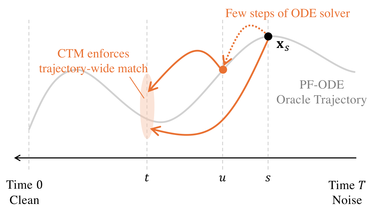
However, solving across the full interval \([t,s]\) during training loop can be costly when \(s\) and \(t\) are far apart. To improve efficiency and provide a smoother signal, CTM introduces soft consistency matching, which operationalizes the semigroup property. As illustrated in Figure 1.5, CTM compares two predictions at time \(t\): the direct student output \(\mathbf{G}_{\bm{\theta}}({\mathbf{x}}_s, s, t)\), and a mixed teacher–student path that first advances the teacher from \(s\) to a random \(u \sim \mathcal{U}[t,s)\), then lets the student jump from \(u\) to \(t\): \[\mathbf{G}_{\bm{\theta}^-} \big(\mathtt{Solver}_{s\to u}({\mathbf{x}}_s;\bm{\phi}^\times),\, u,\, t\big).\] The student is trained to match this composite prediction: \[\begin{align} \label{eq:soft} \underbrace{\mathbf{G}_{\bm{\theta}}({\mathbf{x}}_s, s, t)}_{\approx\, {\bm{\Psi}}_{s\to t}({\mathbf{x}}_s)} \approx \underbrace{\mathbf{G}_{\bm{\theta}^-} \big(\mathtt{Solver}_{s\to u}({\mathbf{x}}_s;\bm{\phi}^\times), u, t\big)}_{\approx\, {\bm{\Psi}}_{u\to t}({\bm{\Psi}}_{s\to u}({\mathbf{x}}_s))}, \end{align}\] where \(\bm{\theta}^-\) is a stop gradient copy of \(\mathbf{G}_{\bm{\theta}}\).
By varying \(u\), CTM interpolates between global and local supervision:
Global Consistency (\(u=t\)): the teacher is solved over the full interval \(s\to t\), so the target reduces to the full teacher transition at time \(t\).
Local Consistency (\(u=s-\Delta s\)): the student learns from a short teacher step near \(s\); when \(t=0\), this reduces to consistency distillation.
To reinforce sample quality while aligning trajectories, both predictions are mapped to time \(0\) by the stop gradient student and compared in a feature space metric \(d\): \[\begin{align*} {\mathbf{x}}_{\mathrm{est}}({\mathbf{x}}_s,s,t) &:= \mathbf{G}_{\bm{\theta}^-} \big(\mathbf{G}_{\bm{\theta}}({\mathbf{x}}_s,s,t),\, t,\, 0\big),\\ {\mathbf{x}}_{\mathrm{target}}({\mathbf{x}}_s,s,u,t) &:= \mathbf{G}_{\bm{\theta}^-} \big( \mathbf{G}_{\bm{\theta}^-}(\mathtt{Solver}_{s\to u}({\mathbf{x}}_s;\bm{\phi}^\times), u, t),\, t,\, 0\big). \end{align*}\] The CTM consistency loss is
\[\begin{align} \label{eq:ctm-consist-distill} \begin{aligned} \mathcal{L}_{\mathrm{consist}}(\bm{\theta}; \bm{\phi}^\times) := \mathbb{E}_{s \in [0,T]}\mathbb{E}_{t \in [0,s]}\mathbb{E}_{u \in [t,s)} \mathbb{E}_{{\mathbf{x}}_0}\mathbb{E}_{{\mathbf{x}}_s |{\mathbf{x}}_0} \Big[ d\big({\mathbf{x}}_{\mathrm{est}}, {\mathbf{x}}_{\mathrm{target}}\big) \Big], \end{aligned} \end{align}\]
which encourages the student to match the empirical PF-ODE solution while preserving generation quality.
Training from Scratch.
Leveraging CTM’s special parameterization (Proposition: Properties of ^*(i)), \[{\mathbf{g}}^*({\mathbf{x}}_\tau, \tau, \tau) = {\mathbf{x}}_\tau - \tau\,{\mathbf{v}}^*({\mathbf{x}}_\tau,\tau) \implies {\mathbf{v}}^*({\mathbf{x}}_\tau,\tau) = \frac{{\mathbf{x}}_\tau - {\mathbf{g}}^*({\mathbf{x}}_\tau, \tau, \tau)}{\tau}.\] We can therefore replace the oracle residual function \({\mathbf{g}}^*(\cdot,\tau,\tau)\) with CTM’s own estimate \({\mathbf{g}}_{\bm{\theta}^-}(\cdot,\tau,\tau)\) for \(\tau \in (0,T]\), which yields a self-induced empirical PF-ODE: \[\begin{align} \label{eq:emp-pf-ode-ctm} \frac{\mathop{}\!\mathrm{d}{\mathbf{x}}(\tau)}{\mathop{}\!\mathrm{d}\tau} = \frac{{\mathbf{x}}(\tau) - {\mathbf{g}}_{\bm{\theta}^-} \left({\mathbf{x}}(\tau),\tau,\tau\right)}{\tau}. \end{align}\]
We then solve this self-induced ODE to construct a tractable transition target: \[\mathbf{G}_{\bm{\theta}}({\mathbf{x}}_s, s, t) \approx \mathtt{Solver}_{s\to t}({\mathbf{x}}_s;\bm{\theta}^-).\] This target approaches the oracle flow map only insofar as the diagonal estimate \({\mathbf{g}}_{\bm{\theta}^-}(\cdot,\tau,\tau)\) accurately recovers the target local dynamics. The diffusion-model loss introduced below provides direct supervision for this local quantity.
As in the distillation case Equation \(\eqref{eq:soft}\), full integration over \([t,s]\) can be costly when \(s\) and \(t\) are far apart. CTM therefore enforces the semigroup property to obtain a shorter supervision path: \[\underbrace{\mathbf{G}_{\bm{\theta}}({\mathbf{x}}_s, s, t)}_{\approx\, {\bm{\Psi}}_{s\to t}({\mathbf{x}}_s)} \approx \underbrace{\mathbf{G}_{\bm{\theta}^-} \big(\mathtt{Solver}_{s\to u}({\mathbf{x}}_s;\bm{\theta}^-),\, u,\, t\big)}_{\approx\, {\bm{\Psi}}_{u\to t}({\bm{\Psi}}_{s\to u}({\mathbf{x}}_s))},\] where \(u \sim \mathcal{U}[t,s)\) and \(\bm{\theta}^-\) is a stop gradient copy of the student. The only change from distillation is that the external teacher \({\mathbf{v}}_{\bm{\phi}^\times}\) is replaced by the self-induced teacher \({\mathbf{g}}_{\bm{\theta}^-}\).
To couple trajectory matching with sample quality, both predictions are mapped to time \(0\) using the stop gradient student and compared in feature space. The target without any pre-trained model is \[\hat{{\mathbf{x}}}_{\mathrm{target}} := \mathbf{G}_{\bm{\theta}^-} \big( \mathbf{G}_{\bm{\theta}^-}(\mathtt{Solver}_{s\to u}({\mathbf{x}}_s;\bm{\theta}^-),\, u,\, t),\, t,\, 0\big),\] which replaces \({\mathbf{x}}_{\mathrm{target}}\) in Equation \(\eqref{eq:ctm-consist-distill}\), and leads to:
\[\begin{align} \label{eq:ctm-consist-scratch} \begin{aligned} \mathcal{L}_{\mathrm{consist}}(\bm{\theta}; {\bm{\theta}}^-) := \mathbb{E}_{s \in [0,T]}\mathbb{E}_{t \in [0,s]}\mathbb{E}_{u \in [t,s)} \mathbb{E}_{{\mathbf{x}}_0}\mathbb{E}_{{\mathbf{x}}_s |{\mathbf{x}}_0} \Big[ d\big({\mathbf{x}}_{\mathrm{est}}, \hat{\mathbf{x}}_{\mathrm{target}}\big) \Big], \end{aligned} \end{align}\]
Conceptually, this is self-distillation within CTM: the model supplies its own short horizon teacher signals while the student learns the full transition.
Auxiliary Losses in CTM
(Self-)distillation can underperform the teacher because it optimizes only teacher generated targets, lacking direct supervision from real data. By contrast, CTM can naturally incorporate data driven regularizers, for example by augmenting its objective with denoising score matching and an adversarial (GAN) term (Goodfellow et al. 2014), to better learn the flow map.
Natural Integration of Diffusion Loss.
The diffusion–model loss (more precisely, the conditional flow matching loss; see Equation in Chapter 5) integrates naturally into CTM and provides a fixed regression target that facilitates the learning of the flow map model. To see this, note that we have \[{\mathbf{v}}^*({\mathbf{x}}_s, s) = \frac{{\mathbf{x}}_s - {\mathbf{g}}^*({\mathbf{x}}_s, s, s)}{s}, \qquad {\mathbf{g}}^*({\mathbf{x}}_s, s, s) \approx {\mathbf{g}}_{{\bm{\theta}}}({\mathbf{x}}_s, s, s).\] This naturally induces a velocity parametrization through \({\mathbf{g}}_{{\bm{\theta}}}\): \[{\mathbf{v}}_{{\bm{\theta}}}({\mathbf{x}}_s, s) := \frac{1}{s}\bigl({\mathbf{x}}_s - {\mathbf{g}}_{{\bm{\theta}}}({\mathbf{x}}_s, s, s)\bigr).\] Using the linear Gaussian path \[{\mathbf{x}}_s = \alpha_s {\mathbf{x}}_0 + \sigma_s {\bm{\epsilon}}, \qquad {\mathbf{x}}_0 \sim p_{\mathrm{data}}, {\bm{\epsilon}}\sim \mathcal N(0, \mathbf I),\] the diffusion model loss can be written as \[\begin{align} \label{eq:ctm-dsm} \mathcal L_{\mathrm{DM}}({\bm{\theta}}) &:= \mathbb{E}_{{\mathbf{x}}_0, {\bm{\epsilon}}, s} \Bigl[ w(s) \bigl\| {\mathbf{v}}_{{\bm{\theta}}}({\mathbf{x}}_s, s) - \left(\alpha_s' {\mathbf{x}}_0 + \sigma_s' {\bm{\epsilon}}\right) \bigr\|_2^2 \Bigr]. \end{align}\]
\(\mathcal L_{\mathrm{DM}}\) improves accuracy when \(t\) is close to \(s\) by explicitly supervising small jumps along the trajectory. In this regime, the factor \(1-\tfrac{t}{s}\) in Equation \(\eqref{eq:ctm_para_1}\) approaches zero, which can weaken gradients and slow learning; \(\mathcal L_{\mathrm{DM}}\) supplies a stronger local signal and stabilizes training.
Conceptually, Equation and Equation enforce trajectory matching (zeroth order), while Equation \(\eqref{eq:ctm-dsm}\) enforces slope matching (first order).
(Optional) GAN Loss.
While consistency and diffusion model loss provide strong regression signals, they can yield overly smooth outputs. CTM therefore optionally adds an adversarial term to encourage sharper, more realistic samples by aligning the generator distribution with the data distribution. With a discriminator \(D_{\bm{\zeta}}\) that distinguishes real \({\mathbf{x}}_{0}\sim p_{\mathrm{data}}\) from generated \({\mathbf{x}}_{\mathrm{est}}({\mathbf{x}}_{s},s,t)\), the objective is \[\begin{align*} &\mathcal{L}_{\mathrm{GAN}}(\bm{\theta}, \bm{\zeta}) := \\ &\mathbb{E}_{\mathbf{x}_0} \big[\log D_{\bm{\zeta}}(\mathbf{x}_0)\big] + \mathbb{E}_{s \in [0, T]} \mathbb{E}_{t \in [0, s]} \mathbb{E}_{\mathbf{x}_0} \mathbb{E}_{\mathbf{x}_s \vert \mathbf{x}_0} \big[\log (1 - D_{\bm{\zeta}}( \mathbf{x}_{\mathrm{est}}(\mathbf{x}_s, s, t)))\big], \end{align*}\] where \(D_{\bm{\zeta}}\) is maximized and \({\mathbf{G}}_{\bm{\theta}}\) is minimized. Intuitively, the discriminator acts as an adaptive perceptual distance that encourages realistic detail. Theoretically, the GAN term drives distributional matching (Jensen–Shannon divergence) between \(p_{\mathrm{data}}\) and the model distribution induced by \({\mathbf{G}}_{\bm{\theta}}\) (Goodfellow et al. 2014), which can raise fidelity beyond the teacher.
Overall CTM Objective.
In summary, CTM unifies (self-)distillation, diffusion, and GAN losses into a single training framework:
\[\begin{align*} \mathcal{L}_{\mathrm{CTM}}(\bm{\theta},\bm{\zeta}) := \mathcal{L}_{\mathrm{consist}}(\bm{\theta}; \bm{\phi}^\times/\bm{\theta}^-) + \lambda_{\mathrm{DM}} \mathcal{L}_{\mathrm{DM}}(\bm{\theta}) + \lambda_{\mathrm{GAN}} \mathcal{L}_{\mathrm{GAN}}(\bm{\theta},\bm{\zeta}), \end{align*}\]
where the teacher is either an external pre-trained model \(\bm{\phi}^\times\) or the self-induced teacher \(\bm{\theta}^-\). The regression style components \(\mathcal{L}_{\mathrm{consist}}\) and \(\mathcal{L}_{\mathrm{DM}}\) act as strong regularizers, while the optional GAN term improves fine scale detail without sacrificing stability (Kim, Lai, Liao, Takida, et al. 2024).
Flexible Sampling with CTM
CTM learns the general flow map \({\bm{\Psi}}_{s\to t}\) for any \(s>t\), which means it supports anytime to anytime transitions. This property enables flexible sampling strategies. For example, CTM proposes \(\gamma\) sampling, where the hyperparameter \(\gamma\) controls the stochasticity during generation. In addition, CTM can reuse standard inference techniques developed for diffusion models, such as ODE based solvers and exact likelihood computation.
In what follows, we fix a discrete time grid for sampling \(T=\tau_0 > \tau_1 > \tau_2 > \cdots > \tau_{M}=0\).
Algorithm: CTM’s γ-sampling
Input: Trained CTM \(\mathbf{G}_{\bm{\theta}^\times}\), \(\gamma\in[0,1]\), \(T=\tau_0>\tau_1 > \tau_2 > \cdots > \tau_{M}=0\).
Start from \(\mathbf{x}_{\tau_{0}}\sim p_{\mathrm{prior}}=\mathcal{N}(\bm{0}, T^2{\mathbf{I}})\)
for \(n=0\) to \(M-1\) do
\(\tilde{\tau}_{n+1}\leftarrow \sqrt{1-\gamma^{2}}\tau_{n+1}\)
Denoise \(\mathbf{x}_{\tilde{\tau}_{n+1}}\leftarrow \mathbf{G}_{\bm{\theta}^\times}(\mathbf{x}_{\tau_{n}},\tau_{n},\tilde{\tau}_{n+1})\)
Diffuse \(\mathbf{x}_{\tau_{n+1}}\leftarrow\mathbf{x}_{\tilde{\tau}_{n+1}}+\gamma \tau_{n+1}\bm{\epsilon}\), where \(\bm{\epsilon}\sim\mathcal{N}(\bm{0}, {\mathbf{I}})\)
Output: \(\mathbf{x}_{\tau_{M}}\)
Methodology of \(\gamma\)-Sampling.
CTM’s \(\gamma\)-sampling introduces a unified family of samplers that arises naturally from learning a general flow map model. It encompasses prior approaches, such as CM’s multistep sampling (see Algorithm (CM’s Sampling with One-Step or Multi-Step Generation)) and time-stepping-style sampling, which is conceptually similar to ODE solvers. The parameter \(\gamma\) directly controls the degree of semantic change during generation, making \(\gamma\) sampling a flexible and task aware strategy for diverse downstream applications.
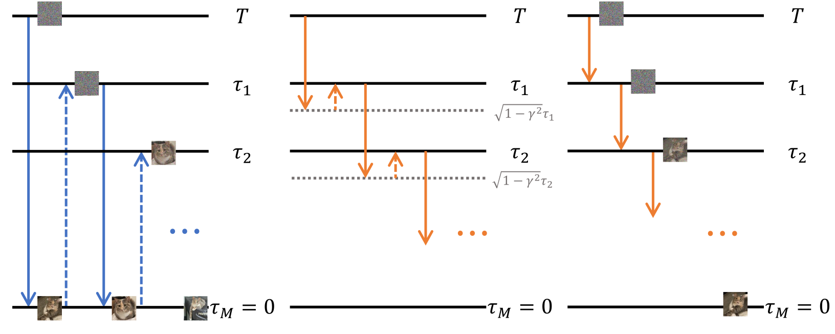
Figure 1.6-(Left): When \(\gamma=1\), it coincides with the multistep sampling introduced in CM (i.e., a special flow map \({\bm{\Psi}}_{s\to 0}\)), which is fully stochastic and results in semantic variation when the number of steps changes.
Figure 1.6-(Right): When \(\gamma=0\), it reduces to fully deterministic time-stepping, which estimates the solution trajectory of the PF-ODE. A key distinction between \(\gamma\) sampling with \(\gamma=0\) and conventional time-stepping ODE-based sampling is that CTM avoids the discretization errors of numerical solvers.
Figure 1.6-(Middle): When \(0 < \gamma < 1\), \(\gamma\)-sampling interpolates between the two extremes by allowing a controlled amount of stochasticity to be injected during sampling.
We highlight that values \(\gamma\in[0,1)\) require the general flow map \({\bm{\Psi}}_{s\to t}\), whereas the special case \(\gamma=1\) reduces to CM-style multistep sampling and requires only \({\bm{\Psi}}_{s\to0}\).
Analysis of \(\gamma\)-Sampling.
CTM empirically observed that CM’s multistep sampling degrades in quality once the number of steps \(M \geq 4\). To explain this phenomenon, CTM analyzed the underlying cause: when \(\gamma \neq 0\), each neural “jump” introduces a small mismatch, and these mismatches accumulate as the model iteratively maps states toward time zero. This error accumulation explains why long multi-step runs can perform poorly. We formalize this idea in the following proposition.
Proposition: (Informal) 2-step \(\gamma\)-sampling
Let \(\tau\in(0,T)\) and \(\gamma \in [0,1]\). Let \(p_{\bm{\theta}^{*},2}\) denote as the density obtained from the \(\gamma\)-sampler with the optimal CTM, following the transition sequence \(T\rightarrow\sqrt{1-\gamma^2}\tau\rightarrow \tau \rightarrow 0\), starting from \(p_T\). Then \[\begin{align*} \mathcal D_{\mathrm{TV}}\big( p_{\mathrm{data}}, p_{\bm{\theta}^{*},2} \big) = \mathcal{O}\left(\sqrt{T-\sqrt{1-\gamma^2}\tau+ \tau} \right). \end{align*}\] Here, \(\mathcal{D}_{\mathrm{TV}}\) denotes the total variation between distributions (see Equation in Chapter 1).
Proof for Proposition. We refer the reader to Theorem 8 of Kim, Lai, Liao, Murata, et al. (2024) for the general case when the number of sampling steps is \(M\). ■
The insights from the above theorem can be summarized as follows:
When \(\gamma = 1\) (corresponding to CM’s multistep sampling): The method performs iterative long-range transitions from \(\tau_n\) to \(0\) at each step \(n\). This leads to error accumulation on the order of \[\begin{align*} \mathcal{O}\left(\sqrt{T + \tau_1 + \cdots + \tau_M}\right). \end{align*}\]
When \(\gamma = 0\) (corresponding to CTM’s deterministic multistep sampling): Such temporal overlap between transitions is eliminated. This avoids error accumulation and yields a tighter bound of \(\mathcal{O}(\sqrt{T})\). Empirically, CTM with \(\gamma = 0\) provides a favorable trade-off between sampling speed and sample quality: increasing the number of sampling steps improves generation quality without introducing instability.
CTM Supports Diffusion Inference.
Since CTM learns the score function (or denoiser) directly through \({\mathbf{g}}_{\bm{\theta}}\), thanks to its parametrization in Equation \(\eqref{eq:ctm_para_1}\), it is compatible with inference techniques originally developed for diffusion models. For instance, one can compute exact likelihoods (Section (Sampling and Inference) in Chapter 4) or apply advanced samplers such as DDIM or DPM (Chapter 9) for generation, by using \({\mathbf{g}}_{\bm{\theta}}(\cdot, s, s)\).
General Flow Map: Mean Flow
Just as diffusion models admit many equivalent parameterizations and training objectives, a general flow map \({\bm{\Psi}}_{s\to t}\) can also be learned in multiple plausible ways. In this section, we introduce Mean Flow (MF) (Geng, Deng, et al. 2025), a later representative of the general flow map family \({\bm{\Psi}}_{s\to t}\) that illustrates an alternative yet principled perspective on how such maps can be effectively learned.
Modeling and Training of Mean Flow
In contrast to CM and CTM, which build on the EDM framework, MF is based on the flow matching formulation (\(\alpha_t = 1-t\) and \(\sigma_t = t\) for \(t\in[0,1]\)). Rather than directly parameterizing the flow map, MF learns the average drift over an interval \([t,s]\) (with \(t<s\)): \[{\mathbf{h}}_{{\bm{\theta}}}({\mathbf{x}}_s, s, t) \approx {\mathbf{h}}^*({\mathbf{x}}_s, s, t) := \frac{1}{t-s}\int_s^t {\mathbf{v}}^*({\mathbf{x}}_u,u) \mathop{}\!\mathrm{d}u.\] The corresponding oracle loss is \[\begin{align} \label{eq:mf-oracle} \mathbb{E}_{t<s} \mathbb{E}_{{\mathbf{x}}_s\sim p_s}\Big[w(s) \|{\mathbf{h}}_{{\bm{\theta}}}({\mathbf{x}}_s,s,t) - {\mathbf{h}}^*({\mathbf{x}}_s,s,t)\|_2^2\Big]. \end{align}\] In particular, when \(s \to t\), the loss function reduces to the flow matching loss: \[\begin{align} \label{eq:mf-to-fm} \mathbb{E}_{t} \mathbb{E}_{{\mathbf{x}}_t\sim p_t}\Big[w(t) \|{\mathbf{h}}_{{\bm{\theta}}}({\mathbf{x}}_t,t,t) - {\mathbf{v}}^*({\mathbf{x}}_t,t)\|_2^2\Big], \end{align}\] learning the instantaneous velocity. We will see later in Section 1.5.3 that MF remains consistent with the general objective in Equation \(\eqref{eq:general-cm-loss:rep}\), but approaches it from a different (while equivalent) perspective. Since the oracle regression target \({\mathbf{h}}^*({\mathbf{x}}_s,s,t)\) does not admit a closed form in general, MF constructs a surrogate by exploiting an identity obtained from differentiating \[(t-s)\,{\mathbf{h}}^*({\mathbf{x}}_s,s,t) = \int_s^t {\mathbf{v}}^*({\mathbf{x}}_u,u)\,\mathop{}\!\mathrm{d}u\] with respect to \(s\). This yields the MF identity: \[\begin{align} \label{eq:mf-identity} \begin{aligned} {\mathbf{h}}^*({\mathbf{x}}_s,s,t) &= {\mathbf{v}}^*({\mathbf{x}}_s,s) - (s-t) \tfrac{\mathop{}\!\mathrm{d}}{\mathop{}\!\mathrm{d}s}{\mathbf{h}}^*({\mathbf{x}}_s,s,t) \\ &= {\mathbf{v}}^*({\mathbf{x}}_s,s) - (s-t)\Big[(\partial_{{\mathbf{x}}}{\mathbf{h}}^*)({\mathbf{x}}_s,s,t) {\mathbf{v}}^*({\mathbf{x}}_s,s) + \partial_s {\mathbf{h}}^*({\mathbf{x}}_s,s,t)\Big], \end{aligned} \end{align}\] where the second line applies the chain rule together with \[\frac{\mathop{}\!\mathrm{d}}{\mathop{}\!\mathrm{d}s}{\mathbf{x}}_s = {\mathbf{v}}^*({\mathbf{x}}_s,s).\]
Motivated by this identity, MF replaces the intractable oracle with a stop-gradient surrogate, leading to the practical training objective
\[\begin{align} \label{eq:mf-practice} \mathcal{L}_{\mathrm{MF}}({\bm{\theta}}) := \mathbb{E}_{t<s} \mathbb{E}_{{\mathbf{x}}_s\sim p_s}\Big[w(s)\, \|{\mathbf{h}}_{{\bm{\theta}}}({\mathbf{x}}_s,s,t) - {\mathbf{h}}_{{\bm{\theta}}^-}^{\mathrm{tgt}}({\mathbf{x}}_s,s,t)\|_2^2\Big], \end{align}\]
where the regression target is defined as \[\begin{align*} {\mathbf{h}}_{{\bm{\theta}}^-}^{\mathrm{tgt}}&({\mathbf{x}}_s,s,t) := \\ &{\mathbf{v}}^*({\mathbf{x}}_s,s) - (s-t)\Big[\underbrace{(\partial_{{\mathbf{x}}}{\mathbf{h}}_{{\bm{\theta}}^-})({\mathbf{x}}_s,s,t) {\mathbf{v}}^*({\mathbf{x}}_s,s) + \partial_s {\mathbf{h}}_{{\bm{\theta}}^-}({\mathbf{x}}_s,s,t)}_{\mathrm{JVP}}\Big]. \end{align*}\]
In practice, the oracle velocity \({\mathbf{v}}^*\) cannot be computed in closed form and must instead be approximated. Two common strategies are available: relying on a pre-trained diffusion model (distillation) or constructing a direct estimator from data (training from scratch). Regardless of the choice, one ultimately needs to compute a Jacobian–vector product (JVP) of the target network \({\mathbf{h}}_{{\bm{\theta}}^-}\): \[\left[\partial_{\mathbf{x}}{\mathbf{h}}_{{\bm{\theta}}^-}, \partial_s {\mathbf{h}}_{{\bm{\theta}}^-}, \partial_t {\mathbf{h}}_{{\bm{\theta}}^-}\right]^\top \cdot \left[{\mathbf{v}}^*, 1, 0\right]\]
Distillation.
Use a pre-trained diffusion model with a flow matching backbone, \({\mathbf{v}}_{{\bm{\phi}}^\times} \approx {\mathbf{v}}^*\).
Training from scratch.
Use the one point conditional velocity \(\alpha_s'{\mathbf{x}}_0 + \sigma_s'{\bm{\epsilon}}\), obtained from the forward noise injection \({\mathbf{x}}_s=\alpha_s{\mathbf{x}}_0+\sigma_s{\bm{\epsilon}}\) with \({\bm{\epsilon}}\sim\mathcal N(\bm{0},{\mathbf{I}})\). This gives an unbiased single sample estimate of the instantaneous drift at level \(s\) when evaluated at paired \(({\mathbf{x}}_0,{\bm{\epsilon}})\).
Sampling of Mean Flow
Once a MF \({\mathbf{h}}_{{\bm{\theta}}^\times}\) is trained, it naturally recovers a proxy of the flow map. For any starting point \({\mathbf{x}}_s\), the map from \(s\) to \(t\) is (approximately) given by \[{\bm{\Psi}}_{s\to t}({\mathbf{x}}_s) = {\mathbf{x}}_s + (t-s)\,{\mathbf{h}}^*({\mathbf{x}}_s,s,t) \approx {\mathbf{x}}_s + (t-s)\,{\mathbf{h}}_{{\bm{\theta}}^\times}({\mathbf{x}}_s,s,t).\]
This enables both one-step and multi-step sampling. For example, drawing \({\mathbf{x}}_T\sim p_{\mathrm{prior}}\), the one-step generation of a clean sample is \[{\mathbf{x}}_0 \leftarrow {\mathbf{x}}_T - T\,{\mathbf{h}}_{{\bm{\theta}}^\times}({\mathbf{x}}_T,T,0).\]
Alternatively, multi-step generation can be performed by preparing a time grid and applying the map sequentially, in the same time-stepping manner used in CTM. Since MF learns a general flow map, it also supports \(\gamma\)-sampling as in CTM, where a controllable hyperparameter \(\gamma\) injects stochasticity into the sampling process.
Relationship between CTM and MF
At first sight CTM and MF may appear unrelated. In fact, both provide different parameterizations of the same oracle flow map \({\bm{\Psi}}_{s\to t}\), and their corresponding squared oracle regression errors are related by a time-dependent weighting (Hu et al. 2025).
Relationship of Parameterizations.
Both methods operate under the same general framework but represent the learned function in distinct ways. The flow map can be written equivalently as \[\begin{align*} {\bm{\Psi}}_{s\to t}({\mathbf{x}}_s) & = {\mathbf{x}}_s + \int_s^t {\mathbf{v}}^*({\mathbf{x}}_u, u)\mathop{}\!\mathrm{d}u \\ &= \frac{t}{s}{\mathbf{x}}_s + \frac{s-t}{s}\underbrace{\Bigg[{\mathbf{x}}_s + \frac{s}{s-t}\int_s^t {\mathbf{v}}^*({\mathbf{x}}_u,u)\,\mathop{}\!\mathrm{d}u\Bigg]}_{\approx\,{\mathbf{g}}_{\bm{\theta}}} \\ &= {\mathbf{x}}_s + (t-s)\underbrace{\Bigg[\frac{1}{t-s}\int_s^t {\mathbf{v}}^*({\mathbf{x}}_u,u)\,\mathop{}\!\mathrm{d}u\Bigg]}_{\approx\,{\mathbf{h}}_{\bm{\theta}}}. \end{align*}\] Here, the first is the definition of the flow map, the second form highlights the CTM parametrization through \({\mathbf{g}}_{\bm{\theta}}\) (see Equation and Equation), while the last highlights the MF parametrization through \({\mathbf{h}}_{\bm{\theta}}\).
Relationship of Training Loss.
Given the above reinterpretation of the oracle flow map \({\bm{\Psi}}_{s\to t}\) in terms of the CTM parametrization \[{\mathbf{g}}_{\bm{\theta}}({\mathbf{x}}_s,s,t) \approx {\mathbf{g}}^*({\mathbf{x}}_s,s,t):={\mathbf{x}}_s + \frac{s}{s-t}\int_s^t {\mathbf{v}}^*({\mathbf{x}}_u,u) \mathop{}\!\mathrm{d}u\] and the MF parametrization \[{\mathbf{h}}_{\bm{\theta}}({\mathbf{x}}_s,s,t) \approx {\mathbf{h}}^*({\mathbf{x}}_s,s,t):=\frac{1}{t-s}\int_s^t {\mathbf{v}}^*({\mathbf{x}}_u,u) \mathop{}\!\mathrm{d}u,\] we now show that the training losses of CTM and MF are in fact equivalent.
Consider the relation \[{\mathbf{g}}_{\bm{\theta}}({\mathbf{x}}_s,s,t) := {\mathbf{x}}_s - s {\mathbf{h}}_{\bm{\theta}}({\mathbf{x}}_s,s,t),\] and take \(d({\mathbf{x}},{\mathbf{y}}):=\|{\mathbf{x}}-{\mathbf{y}}\|^2\) as an example. Substituting into Equation \(\eqref{eq:general-cm-loss:rep}\) and viewing \({\mathbf{G}}_{\bm{\theta}}\) as CTM’s flow-map parameterization (Equation \(\eqref{eq:ctm_para_1}\)) gives \[\begin{align} &~d\big({\mathbf{G}}_{\bm{\theta}}({\mathbf{x}}_s,s,t), {\bm{\Psi}}_{s\to t}({\mathbf{x}}_s)\big) \notag \\ = &~\left\lVert{\mathbf{G}}_{\bm{\theta}}({\mathbf{x}}_s,s,t) - {\bm{\Psi}}_{s\to t}({\mathbf{x}}_s)\right\rVert^2 \notag \\ = &~\left\lVert\left(\frac{t}{s}{\mathbf{x}}_s + \frac{s-t}{s} {\mathbf{g}}_{\bm{\theta}}({\mathbf{x}}_s,s,t)\right)-\left(\frac{t}{s}{\mathbf{x}}_s + \frac{s-t}{s}\Big[{\mathbf{x}}_s + \frac{s}{s-t}\int_s^t {\mathbf{v}}^*({\mathbf{x}}_u,u) \mathop{}\!\mathrm{d}u\Big]\right)\right\rVert^2 \notag \\ = &~\left(\frac{s-t}{s}\right)^2\left\lVert{\mathbf{g}}_{\bm{\theta}}({\mathbf{x}}_s,s,t)-\left({\mathbf{x}}_s + \frac{s}{s-t}\int_s^t {\mathbf{v}}^*({\mathbf{x}}_u,u) \mathop{}\!\mathrm{d}u\right)\right\rVert^2 \label{eq:g-para} \\ = &~\left(\frac{s-t}{s}\right)^2\left\lVert\left({\mathbf{x}}_s - s {\mathbf{h}}_{\bm{\theta}}({\mathbf{x}}_s,s,t)\right)-\left({\mathbf{x}}_s + \frac{s}{s-t}\int_s^t {\mathbf{v}}^*({\mathbf{x}}_u,u) \mathop{}\!\mathrm{d}u\right)\right\rVert^2 \notag \\ = &~\left(\frac{s-t}{s}\right)^2\left\lVert\left({\mathbf{x}}_s - s {\mathbf{h}}_{\bm{\theta}}({\mathbf{x}}_s,s,t)\right)-\left({\mathbf{x}}_s + \frac{s}{s-t}\int_s^t {\mathbf{v}}^*({\mathbf{x}}_u,u) \mathop{}\!\mathrm{d}u\right)\right\rVert^2 \notag \\ = &~\left(s-t\right)^2\left\lVert {\mathbf{h}}_{\bm{\theta}}({\mathbf{x}}_s,s,t)- \left(\frac{1}{t-s}\int_s^t {\mathbf{v}}^*({\mathbf{x}}_u,u)\mathop{}\!\mathrm{d}u \right)\right\rVert^2 \label{eq:h-para} \end{align}\] Hence, \[\begin{align*} \frac{1}{s^2} \Bigg\|{\mathbf{g}}_{\bm{\theta}}({\mathbf{x}}_s,s,t)-{\mathbf{g}}^*({\mathbf{x}}_s,s,t) \Bigg\|^2 = \Bigg\|{\mathbf{h}}_{\bm{\theta}}({\mathbf{x}}_s,s,t)-{\mathbf{h}}^*({\mathbf{x}}_s,s,t) \Bigg\|^2. \end{align*}\] Putting aside the specific algorithm used to learn the flow map, the CTM and MF losses share the same mathematical form, differing only by a weighting function. Moreover, setting \(t=0\) in either case recovers the CM setting (\({\bm{\Psi}}_{s\to 0}\)), where each state maps directly to the clean data.
Auxiliary Loss in Practice.
In CTM, training is performed with the consistency loss in Equation \(\eqref{eq:ctm-consist-scratch}\) jointly with its self-defined diffusion model loss in Equation \(\eqref{eq:ctm-dsm}\). A similar strategy is adopted in MF. As shown in Equation \(\eqref{eq:mf-to-fm}\), when \(s \to t\), the MF loss reduces to the standard flow matching objective. In practice, MF controls the ratio between pairs with \(s \neq t\) and those with \(s = t\); consequently, the overall optimization becomes a mixture of the MF objective in Equation \(\eqref{eq:mf-practice}\) and the flow matching objective in Equation \(\eqref{eq:mf-to-fm}\).
Both parametrizations are able to provide a smooth transition from diffusion-model training, which learns instantaneous velocity with a fixed regression target, to flow-map learning, which employs a stop-gradient pseudo-regression target.
Both CTM and MF Parameterizations Enable Flexible Inference.
Both CTM (\({\mathbf{G}}_{\bm{\theta}}({\mathbf{x}}_s,s,t)\)) and MF (\({\mathbf{h}}_{\bm{\theta}}({\mathbf{x}}_s,s,t)\)) aim to approximate the underlying flow map \({\bm{\Psi}}_{s\to t}\): \[{\mathbf{G}}_{\bm{\theta}}({\mathbf{x}}_s,s,t)\approx{\bm{\Psi}}_{s\to t},\quad \text{and} \quad {\mathbf{x}}_s+(t-s){\mathbf{h}}_{\bm{\theta}}({\mathbf{x}}_s,s,t)\approx{\bm{\Psi}}_{s\to t}.\] Since both models learn an explicit mapping between any two time steps, they naturally support CTM’s \(\gamma\)-sampling and remain compatible with inference techniques originally developed for diffusion models, such as guidance (Chapter 8), exact likelihood computation (Equation in Chapter 4), and accelerated sampling with higher-order solvers (Chapter 9). This compatibility arises because their parameterizations recover the instantaneous diffusion drift in the infinitesimal limit \(t\to s\): \[{\mathbf{g}}^*({\mathbf{x}}_s,s,s)={\mathbf{x}}_s-s\,{\mathbf{v}}^*({\mathbf{x}}_s,s), \quad \text{and} \quad {\mathbf{h}}^*({\mathbf{x}}_s,s,s)={\mathbf{v}}^*({\mathbf{x}}_s,s).\] This property is not shared by specialized flow map formulations \({\bm{\Psi}}_{s\to0}\), such as those in the CM family. Thus, both CTM and MF can be regarded as flexible and general flow map formulations that generalize diffusion-based inference to direct time-to-time mappings.
Conclusion.
The relationship between CTM and MF is analogous to the relationship between different parametrizations of diffusion models (Section (Equivalence in Diffusion Models) in Chapter 6): at the oracle level, they encode the same underlying flow map. Under squared-error regression and the parametrization relation above, their oracle regression errors differ only by a known time-dependent scaling. Their practical training objectives, however, remain different because they use different surrogate targets and optimization procedures.
Although CTM and MF are related in this way, they differ conceptually and algorithmically in how the target is learned. The CTM target is defined in the “integral” form, as it acts directly on the flow map. The MF target, on the other hand, is defined in the “differential” form, as it relies on finite differences of the flow map. Because a target in the integral form is not directly tractable, CTM must solve an ODE during training. In contrast, MF leverages the MF identity (see Equation \(\eqref{eq:mf-identity}\)) to construct a tractable target in the differential form. This relationship is analogous to that between energy-based and score-based methods: the former learns a probability density itself (in the integral form), while the latter matches the gradient of that density (in the differential form). In practice, CTM and MF may behave differently due to factors such as loss weighting, network architecture, and optimization dynamics, which can cause one method to perform better than the other under certain conditions.
This perspective suggests that CTM and MF are not the only viable formulations. Other parameterizations of the flow map could also enable efficient and stable training, potentially leading to new standalone generative models. Exploring these alternatives may further enrich the landscape of diffusion models and their flow map extensions, pushing the boundaries of few-step generation.
Closing Remarks
This final chapter has brought our exploration full circle: from slow iterative diffusion samplers to fast few-step generators (learned from scratch). The common object behind the methods in this chapter is the oracle flow map introduced in Equation \(\eqref{eq:general-cm-loss:rep}\): \[{\bm{\Psi}}_{s\to t}({\mathbf{x}}_s) = {\mathbf{x}}_s+\int_s^t {\mathbf{v}}^*({\mathbf{x}}_\tau,\tau)\,\mathop{}\!\mathrm{d}\tau.\] Learning this map replaces many small numerical updates by one or a few learned jumps.
At this point, it is useful to step back from the individual algorithms. Knowledge Distillation (Section (Prologue) in Chapter 10), Progressive Distillation (Section (Progressive DistillationProgressive Distillation) in Chapter 10), CM (Section 1.2), CTM (Section 1.4), and MF (Section 1.5) were introduced through different training constructions, but they all exploit, explicitly or implicitly, the same ODE solution-map structure.
The flow map itself is a classical object from differential equations and dynamical systems, with closely related particle-based and field-based descriptions in continuum and fluid mechanics; see Equation in Chapter 4 and the surrounding historical discussion. Here, we use three classical descriptions of the same ODE flow, namely the semigroup, Lagrangian, and Eulerian views, as an organizing lens for the modern learning methods developed above 8
Semigroup View: Split the Trip.
As introduced in Equation \(\eqref{eq:semi-group}\), the finite-step identity is \[{\bm{\Psi}}_{u\to t}\big({\bm{\Psi}}_{s\to u}({\mathbf{x}}_s)\big) = {\bm{\Psi}}_{s\to t}({\mathbf{x}}_s).\] As illustrated in Figure 1.3, the intuition is the same as traveling along a fixed route: going from \(s\) to \(u\) and then from \(u\) to \(t\) lands at the same point as going directly from \(s\) to \(t\). Within this view, KD learns the full transition \({\bm{\Psi}}_{T\to0}\), PD compresses two adjacent teacher steps into one student step, CM learns the special anytime-to-clean map \({\bm{\Psi}}_{s\to0}\), and CTM extends the same composition principle to the general map \({\bm{\Psi}}_{s\to t}\).
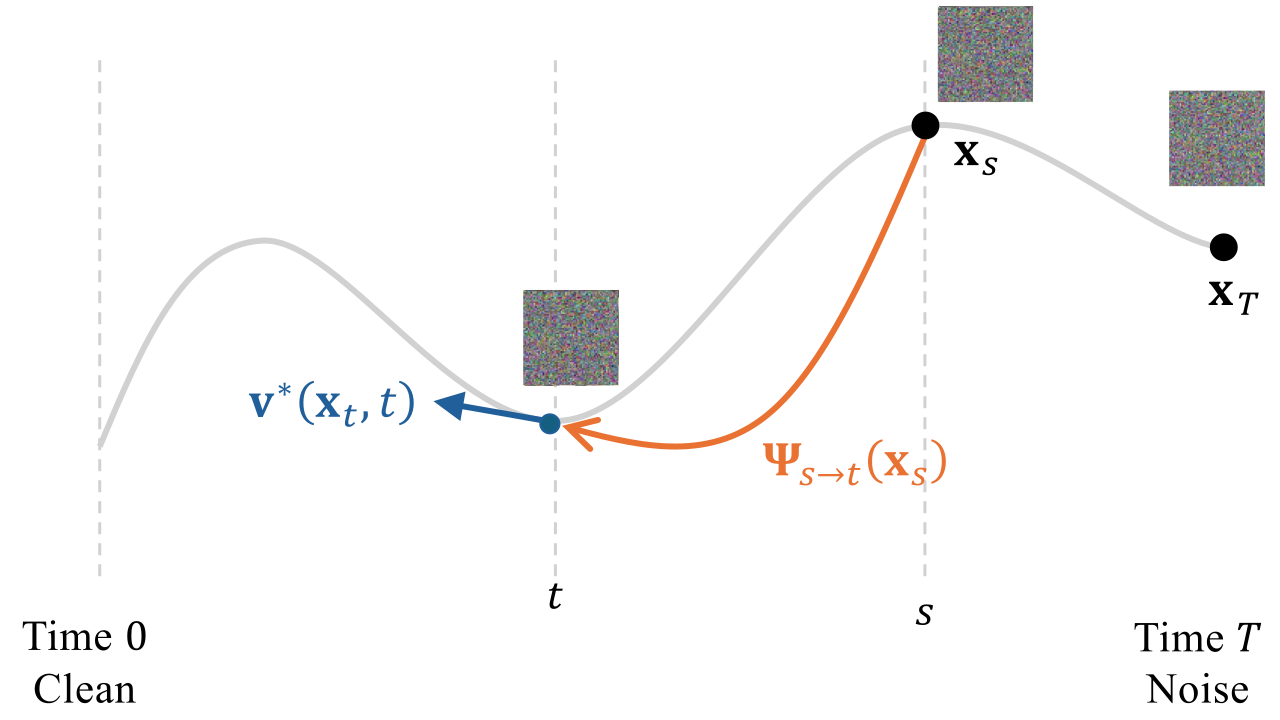
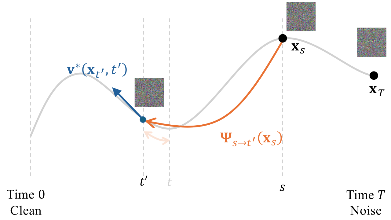
Lagrangian View: Move the Ending Point.
Fix the starting state–time pair \(({\mathbf{x}}_s,s)\) and vary the ending time \(t\). The ending point then moves along the same trajectory: \[\partial_t {\bm{\Psi}}_{s\to t}({\mathbf{x}}_s) = {\mathbf{v}}^*({\bm{\Psi}}_{s\to t}({\mathbf{x}}_s),t).\] The name “Lagrangian” follows the classical particle viewpoint: we track the ending point along the trajectory as the ending time changes. Infinitesimally, the ending point moves with the local ODE velocity evaluated at that point.
Eulerian View: Move the Starting Point.
Fix the ending time \(t\) and slide the starting point along the same trajectory. The ending point at time \(t\) remains fixed: \[\frac{\mathop{}\!\mathrm{d}}{\mathop{}\!\mathrm{d}s}{\bm{\Psi}}_{s\to t}({\mathbf{x}}_s)=0.\] Since \(\frac{\mathop{}\!\mathrm{d}}{\mathop{}\!\mathrm{d}s}{\mathbf{x}}_s={\mathbf{v}}^*({\mathbf{x}}_s,s)\), the chain rule gives \[\partial_s{\bm{\Psi}}_{s\to t}({\mathbf{x}}_s) + \big(\partial_{{\mathbf{x}}}{\bm{\Psi}}_{s\to t}\big)({\mathbf{x}}_s){\mathbf{v}}^*({\mathbf{x}}_s,s) = 0.\] The term “Eulerian” invokes the classical field-based viewpoint: Here, the ending time \(t\) is fixed, while the starting state–time pair \(({\mathbf{x}}_s,s)\) moves along the same ODE trajectory; the ending point at time \(t\) therefore remains unchanged. For CM, the ending time is fixed at \(t=0\), so the ending point is the clean sample: \[{\mathbf{f}}^*({\mathbf{x}}_s,s)={\bm{\Psi}}_{s\to0}({\mathbf{x}}_s).\] Thus, Equation \(\eqref{eq:conti-ct-motivation}\) is the starting-time consistency condition for the special flow map studied in Section (Special Flow Map: Consistency Model in Discrete Time) and Section (Special Flow Map: Consistency Model in Continuous Time).
This view also recaps the relationship between CTM and MF from Section 1.5.3. Both approximate the same path integral \[{\bm{\Psi}}_{s\to t}({\mathbf{x}}_s) = {\mathbf{x}}_s+\int_s^t{\mathbf{v}}^*({\mathbf{x}}_\tau,\tau)\,\mathop{}\!\mathrm{d}\tau,\] but expose different trainable surrogates. CTM represents the ending point through a displacement-style parameterization, while MF represents the same ending point through the average drift \[{\mathbf{h}}^*({\mathbf{x}}_s,s,t) = \frac{1}{t-s}\int_s^t{\mathbf{v}}^*({\mathbf{x}}_\tau,\tau)\,\mathop{}\!\mathrm{d}\tau.\] Substituting \[{\bm{\Psi}}_{s\to t}({\mathbf{x}}_s)={\mathbf{x}}_s+(t-s){\mathbf{h}}^*({\mathbf{x}}_s,s,t)\] into the Eulerian starting-time identity yields \[{\mathbf{h}}^*({\mathbf{x}}_s,s,t) = {\mathbf{v}}^*({\mathbf{x}}_s,s) - (s-t) \left[ \partial_s{\mathbf{h}}^*({\mathbf{x}}_s,s,t) + (\partial_{{\mathbf{x}}}{\mathbf{h}}^*)({\mathbf{x}}_s,s,t){\mathbf{v}}^*({\mathbf{x}}_s,s) \right].\] This is the basic Mean Flow identity: the average drift over a long interval is the instantaneous drift at the starting point, corrected by how the average drift changes as the starting point slides along the same trajectory.
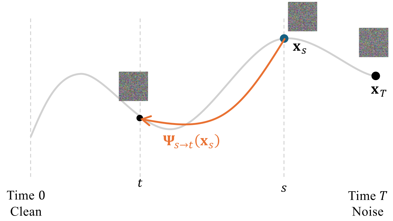
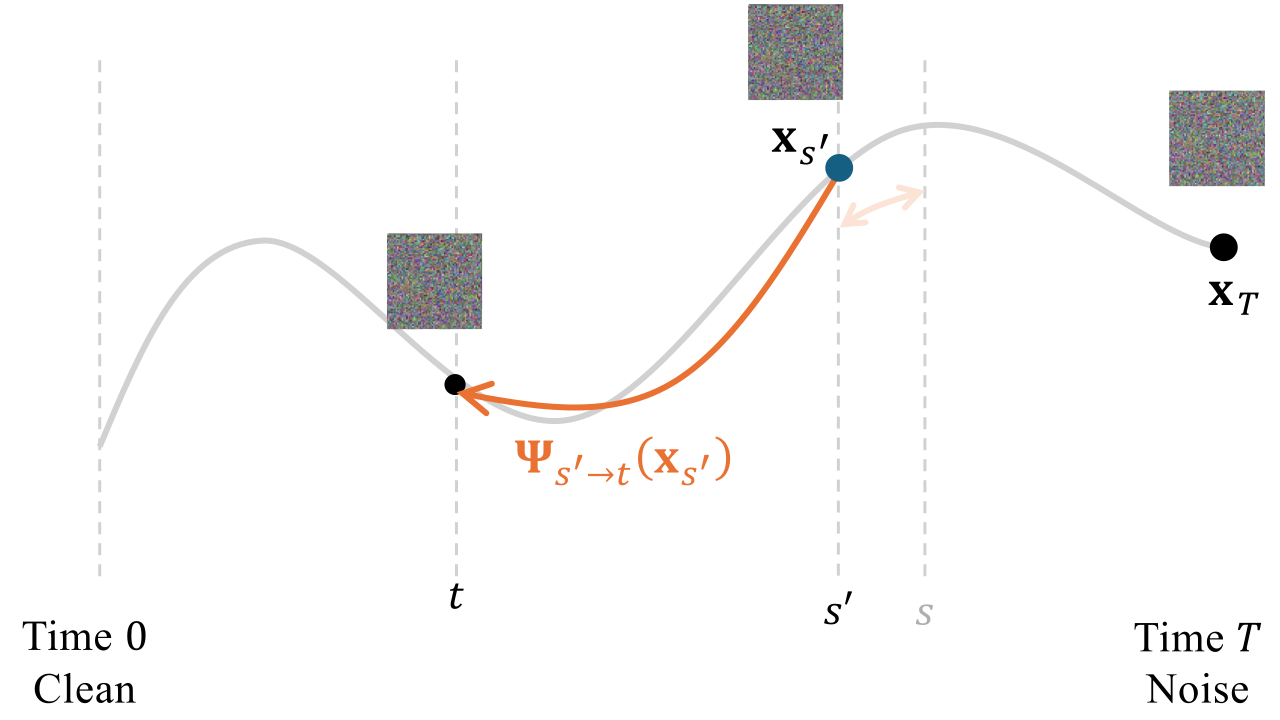
Mathematical Equivalence of the Three Perspectives.
For an exact ODE flow, the semigroup, Lagrangian, and Eulerian identities all express the same simple principle: under standard existence, uniqueness, and smoothness assumptions, an ODE determines a unique trajectory through each state–time pair. That is, once a state at a given time is fixed, there is only one path to follow. The semigroup view splits this path into consecutive pieces, the Lagrangian view follows its ending point as the ending time changes, and the Eulerian view moves the starting point along the same path while keeping the ending point fixed. Thus, the three identities are equivalent descriptions of the same ODE flow (Arnold 1988; Chorin and Marsden 1993). Their connection becomes especially clear by viewing the semigroup identity as the finite-interval statement, and the Lagrangian and Eulerian identities as its two infinitesimal forms, obtained by shrinking a short interval near the ending time or near the starting time, respectively.
The semigroup identity gives the finite-interval form of this principle: \[{\bm{\Psi}}_{u\to t}\big({\bm{\Psi}}_{s\to u}({\mathbf{x}}_s)\big) = {\bm{\Psi}}_{s\to t}({\mathbf{x}}_s), \qquad {\bm{\Psi}}_{s\to s}={\mathbf{I}}.\] The two differential views are obtained by shrinking one of the two intervals.
Ending-Time Limit: the Lagrangian Identity.
Fix the starting state–time pair \(({\mathbf{x}}_s,s)\) and shrink the final segment of the trip. For \(\Delta t>0\), \[{\bm{\Psi}}_{t\to t-\Delta t} \big({\bm{\Psi}}_{s\to t}({\mathbf{x}}_s)\big) = {\bm{\Psi}}_{s\to t-\Delta t}({\mathbf{x}}_s).\] Let \({\mathbf{x}}_t:={\bm{\Psi}}_{s\to t}({\mathbf{x}}_s)\). A first-order expansion of the short flow gives \[{\bm{\Psi}}_{t\to t-\Delta t}({\mathbf{x}}_t) = {\mathbf{x}}_t-\Delta t\,{\mathbf{v}}^*({\mathbf{x}}_t,t) +\mathcal{O}\big((\Delta t)^2\big).\] Therefore, \[\frac{ {\bm{\Psi}}_{s\to t-\Delta t}({\mathbf{x}}_s) - {\bm{\Psi}}_{s\to t}({\mathbf{x}}_s)} {-\Delta t} = {\mathbf{v}}^*({\mathbf{x}}_t,t) +\mathcal{O}(\Delta t).\] Taking \(\Delta t\to0\) yields the Lagrangian identity \[\partial_t{\bm{\Psi}}_{s\to t}({\mathbf{x}}_s) = {\mathbf{v}}^*\big({\bm{\Psi}}_{s\to t}({\mathbf{x}}_s),t\big).\] Thus, when the starting state–time pair \(({\mathbf{x}}_s,s)\) is fixed and the ending time changes, the ending point moves with the ODE velocity evaluated at that point.
Starting-Time Limit: the Eulerian Identity.
Now fix the ending time \(t\) and move the starting state–time pair backward by a short interval \(\Delta s>0\) along the same trajectory: \[{\mathbf{x}}_{s-\Delta s} := {\bm{\Psi}}_{s\to s-\Delta s}({\mathbf{x}}_s) = {\mathbf{x}}_s-\Delta s\,{\mathbf{v}}^*({\mathbf{x}}_s,s) +\mathcal{O}\big((\Delta s)^2\big).\] The semigroup identity gives \[{\bm{\Psi}}_{s-\Delta s\to t}({\mathbf{x}}_{s-\Delta s}) = {\bm{\Psi}}_{s\to t}({\mathbf{x}}_s).\] Expanding the left-hand side in both the starting state and the starting time gives \[{\bm{\Psi}}_{s-\Delta s\to t}({\mathbf{x}}_{s-\Delta s}) = {\bm{\Psi}}_{s\to t}({\mathbf{x}}_s) - \Delta s\, \big(\partial_{{\mathbf{x}}}{\bm{\Psi}}_{s\to t}\big)({\mathbf{x}}_s){\mathbf{v}}^*({\mathbf{x}}_s,s) - \Delta s\, \partial_s{\bm{\Psi}}_{s\to t}({\mathbf{x}}_s) + \mathcal{O}\big((\Delta s)^2\big).\] Comparing with the semigroup identity and dividing by \(-\Delta s\) gives \[\partial_s{\bm{\Psi}}_{s\to t}({\mathbf{x}}_s) + \big(\partial_{{\mathbf{x}}}{\bm{\Psi}}_{s\to t}\big)({\mathbf{x}}_s){\mathbf{v}}^*({\mathbf{x}}_s,s) = \mathcal{O}(\Delta s).\] Taking \(\Delta s\to0\) yields the Eulerian identity \[\partial_s{\bm{\Psi}}_{s\to t}({\mathbf{x}}_s) + \big(\partial_{{\mathbf{x}}}{\bm{\Psi}}_{s\to t}\big)({\mathbf{x}}_s){\mathbf{v}}^*({\mathbf{x}}_s,s) = 0.\] Here, the ending time \(t\) is fixed, while the starting state–time pair moves along the same trajectory. The ending point therefore remains unchanged.
Recovering the Flow Map from Either Differential Identity.
Conversely, either differential identity together with the boundary condition \({\bm{\Psi}}_{s\to s}={\mathbf{I}}\) recovers the same flow map. The Lagrangian identity evolves the ending point from \({\bm{\Psi}}_{s\to s}({\mathbf{x}}_s)={\mathbf{x}}_s\). The Eulerian identity says that \({\bm{\Psi}}_{\tau\to t}({\mathbf{x}}_\tau)\) is constant along the characteristic \({\mathbf{x}}_\tau={\bm{\Psi}}_{s\to \tau}({\mathbf{x}}_s)\), hence \[{\bm{\Psi}}_{s\to t}({\mathbf{x}}_s) = {\bm{\Psi}}_{t\to t}({\mathbf{x}}_t) = {\mathbf{x}}_t.\] Although these perspectives are equivalent at the oracle level, they lead to different practical algorithms once approximations are introduced: one must choose which identity to enforce, where to place stop-gradient targets, how to sample time pairs, and how to parameterize the map.
Closing.
The central shift explored in this chapter is from learning a local velocity field to learning finite pieces of its ODE solution map. A conventional diffusion sampler repeatedly evaluates the local field and numerically integrates it. A flow-map model instead amortizes part of this integration during training, so that a long interval can be traversed with one or a few network evaluations.
This creates a direct route to fast generation, but moves difficulty from sampling into learning. The model must approximate a more global object, and its success depends on the parameterization of the map, the construction of tractable targets, the sampling and weighting of time pairs, and the stabilization of optimization.
Viewed in this way, flow-map learning is not a new dynamical concept but a modern learning strategy built around a classical one. It preserves the trajectory-based foundation of diffusion models while enlarging the design space for efficient generation. The objective is no longer only to integrate the generative ODE more efficiently at inference time, but to learn useful finite-time transitions of its solution map directly.
See Equation in Chapter 4 and the surrounding discussion for the mathematical and historical background of flow maps.↩︎
The semigroup property follows from the uniqueness theorem for ODE initial value problems (see Appendix A).↩︎
The concept of a consistency function for an ODE generalizes to a function \({\mathbf{f}}({\mathbf{x}},t)\) for an SDE such that \({\mathbf{f}}({\mathbf{x}}_t,t)\) is a (local) martingale with respect to the SDE’s natural filtration, i.e. \[\mathbb{E}[{\mathbf{f}}({\mathbf{x}}_t,t)|{\mathbf{x}}_s]={\mathbf{f}}({\mathbf{x}}_s,s),\quad\text{for all }\quad t\ge s.\] This generalization was proposed/observed in (Daras et al. 2023; Lai, Takida, Murata, et al. 2023), and the theoretical connections are summarized in (Lai, Takida, Uesaka, et al. 2023).↩︎
The last identity follows directly from the forward corruption process \({\mathbf{x}}_s=\alpha_s {\mathbf{x}}_0+\sigma_s {\bm{\epsilon}}\) by elementary algebra.↩︎
The one-point (conditional) score estimate \(\widehat{\nabla_{{\mathbf{x}}}\log}p_s({\mathbf{x}}_s)\) can be viewed as a one-sample Monte Carlo estimator, which is conditionally unbiased given \({\mathbf{x}}_s\): averaging this estimator over the (generally intractable) clean posterior \(p(\cdot|{\mathbf{x}}_s)\) recovers the true score as \[\nabla_{{\mathbf{x}}_s}\log p_s({\mathbf{x}}_s) = \mathbb{E}_{{\mathbf{x}}_0\sim p(\cdot|{\mathbf{x}}_s)} \left[\widehat{\nabla_{{\mathbf{x}}}\log}p_s({\mathbf{x}}_s)\right].\]↩︎
Intuitively, both the trigonometric functions and their derivatives are bounded, which helps prevent scale explosion in terms like \(\frac{\mathop{}\!\mathrm{d}}{\mathop{}\!\mathrm{d}s} {\mathbf{f}}_{\bm{\theta}^-}\). A detailed discussion is provided later.↩︎
For affine-in-time schedules, such as \((\alpha_t,\sigma_t)=(1,t)\) or \((1-t,t)\), the plain Euler step in diffusion time coincides exactly with the deterministic DDIM update. For general schedules, the two agree only to first order. See discussion in Section (Relation to Euler-Type Methods) in Chapter 9.↩︎
In modern generative modeling, Boffi et al. (2025) bring together structural ideas that already appear across PD, CM, CTM, and MF, and use them to describe the learning of diffusion PF-ODE flow maps in a common language. The main ingredients therefore largely come from these existing lines of work. Our presentation and illustrations in this part are also informed by the exposition of Dieleman (2026).↩︎