Chapter 5: Flow-Based Perspective: From NFs to Flow Matching
Everything flows.
Heraclitus
The change-of-variables formula, a cornerstone of probability theory (Tabak and Vanden-Eijnden 2010; Turner 2013), takes on new life in modern generative modeling. In Chapter 4, we saw that the Fokker–Planck equation describes how probability densities evolve under a diffusion process, and that the same marginal density evolution can also be realized deterministically through the associated PF-ODE. This naturally suggests studying generative modeling directly from the viewpoint of deterministic probability transport.
Change-of-Variables Formula of Densities.
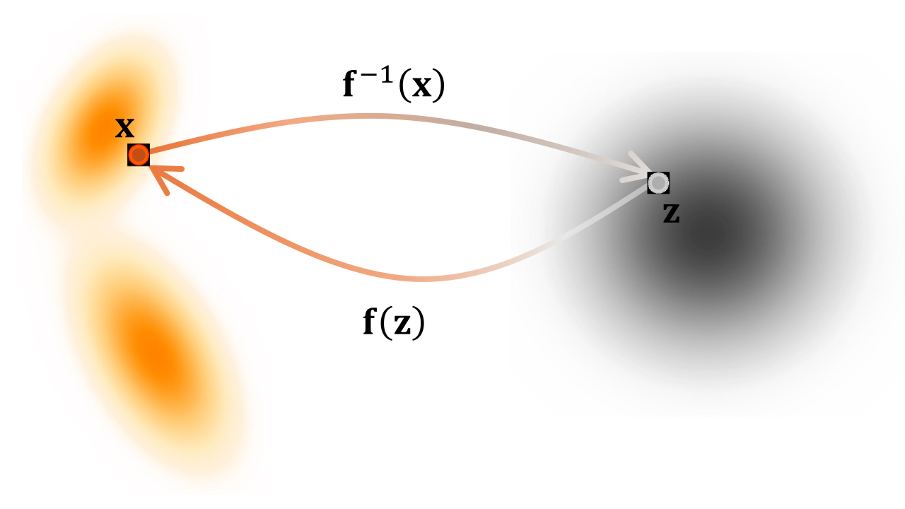
Given an invertible transformation \({\mathbf{f}}\), the density of \({\mathbf{x}}={\mathbf{f}}({\mathbf{z}})\), where \({\mathbf{z}}\sim p_{\mathrm{prior}}\), is
\[\begin{align} \label{eq:nf-change-of-var} p({\mathbf{x}}) = p_{\mathrm{prior}}({\mathbf{z}}) \left| \det \frac{\partial {\mathbf{f}}^{-1}({\mathbf{x}})}{\partial {\mathbf{x}}} \right|, \qquad \text{where } {\mathbf{z}}={\mathbf{f}}^{-1}({\mathbf{x}}). \end{align}\]
This deceptively simple formula enables bidirectional transport of samples and densities when \({\mathbf{f}}\) is tractable, forming the foundation of Normalizing Flows, which we introduce in Section 1.1. But what happens when this transformation is viewed continuously in time?
In this chapter, we follow this idea from Normalizing Flows to Neural ODEs and then to Flow Matching. The key connection to Chapter 4 is especially important. In Score SDEs, the learned score is used to construct the velocity field of the PF-ODE. Flow Matching instead learns a velocity field directly. For the same diffusion probability path, these provide two views of the same deterministic probability flow.
A useful mental picture for this chapter is therefore, where both rely on the same conditioning principle:
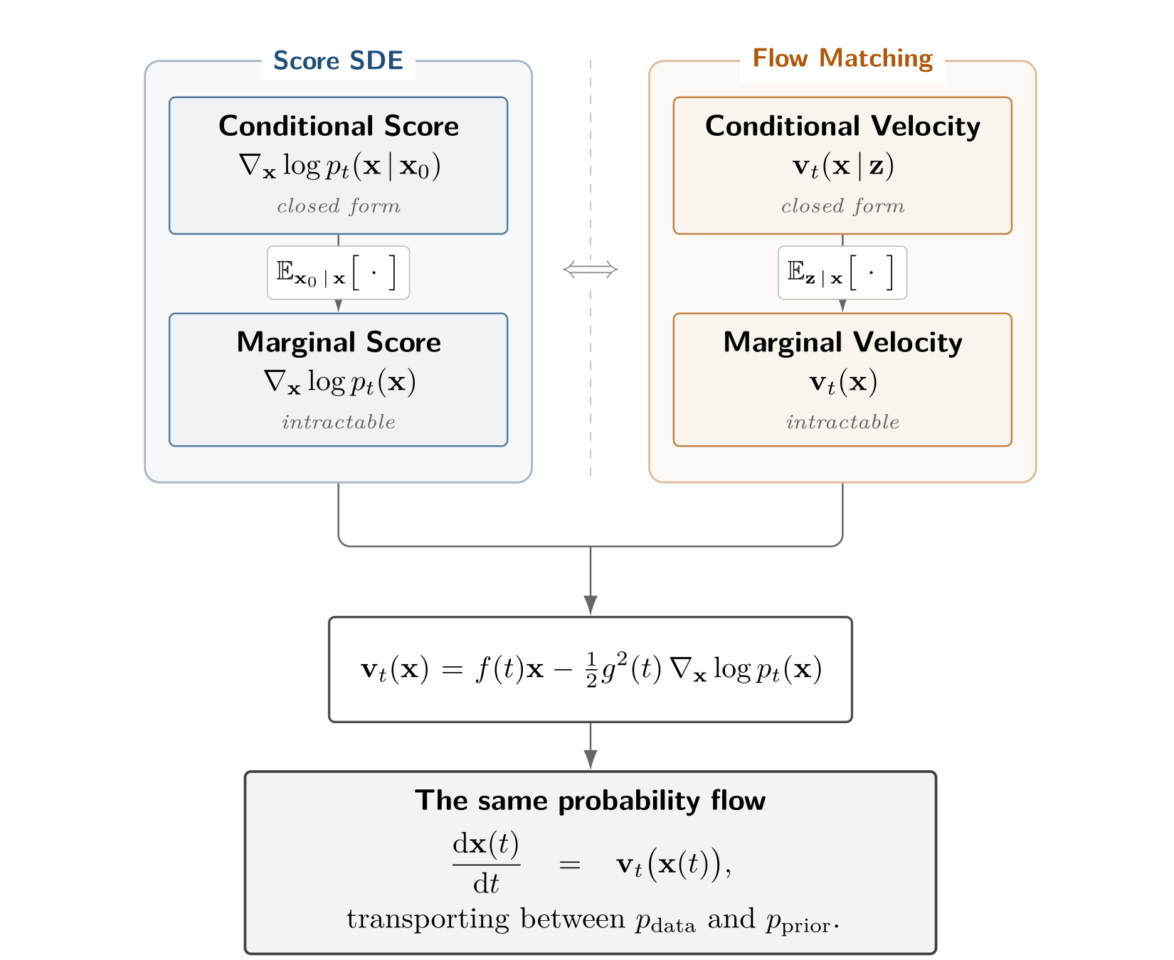
Flow Matching carries this principle beyond the usual Gaussian diffusion setting. It can construct continuous transport between more general source and target distributions from which samples are available, provided that the chosen conditional probability paths can be sampled efficiently and their conditional velocities can be computed tractably.
To support a solid understanding of this chapter, we provide in Appendix B an intuitive, self-contained overview of the different forms of the change-of-variables principle, progressing from the ordinary change-of-variables formula to the continuity equation and, with stochastic dynamics, to the Fokker–Planck equation.
After this chapter, you will be able to...
connect Normalizing Flows, Neural ODEs, and Flow Matching through the common idea of transporting probability distributions, from discrete invertible transformations to continuous-time velocity fields;
recognize the key analogy with the Score SDE framework in Chapter 4: for the same diffusion probability path, Score SDEs learn a score that determines the PF-ODE velocity, whereas Flow Matching can learn that velocity field directly; in both cases, an intractable marginal target can be learned through tractable conditional targets;
understand the continuity equation as the density-level rule that connects an ODE velocity field to the evolution of its probability distribution;
understand how Flow Matching extends this conditional strategy beyond Gaussian diffusion paths to transport between general source and target distributions from which samples are available, while retaining simulation-free training through tractable conditional paths and velocities;
distinguish the prescribed probability path \(\{p_t\}_{t\in[0,1]}\) from the particular velocity field, coupling, and particle trajectories used to realize it, and understand why different flows can share the same marginal distributions;
understand the two complementary ways of constructing tractable conditional flows: starting from a conditional probability path and deriving its velocity, or starting from a conditional flow map and deriving its velocity along trajectories.
Reader route. Readers already comfortable with Normalizing Flows and Neural ODEs may skim Section 1.1 and begin with Section 1.2.1. For a first pass, focus on the connection between the Score SDE and Flow Matching views, the continuity equation, and the conditional-to-marginal velocity construction. The detailed path constructions and optional theoretical properties can be revisited afterward.
Flow-Based Models: Normalizing Flows and Neural ODEs
In this section, we will introduce Flow-Based Models, including Normalizing Flows (NFs) (Rezende and Mohamed 2015) and Neural Ordinary Differential Equations (NODEs) (Chen et al. 2018).
NFs enable flexible and tractable probability density estimation by applying a series of invertible transformations to a simple base distribution. NODEs extend this framework to continuous time, where the transformation is governed by an ODE. By treating the transformations as continuous-time dynamics, NODEs provide a smooth, scalable extension to the NF paradigm.
Normalizing Flows
NFs (Rezende and Mohamed 2015) model a complex data distribution \(p_{\text{data}}({\mathbf{x}})\) by transforming a simple prior \(p_{\text{prior}}({\mathbf{z}})\) (e.g., standard Gaussian \(\mathcal{N}(\bm{0}, {\mathbf{I}})\)) via an invertible mapping \[{\mathbf{f}}_{\bm{\phi}}: \mathbb{R}^D \to \mathbb{R}^D,\] with \({\mathbf{x}}= {\mathbf{f}}_{\bm{\phi}}({\mathbf{z}})\) and \({\mathbf{z}}\sim p_{\text{prior}}\). Here, \({\mathbf{x}}\) and \({\mathbf{z}}\) share the same dimension. Using the change-of-variables formula in Equation \(\eqref{eq:nf-change-of-var}\), the model likelihood is1 \[\begin{align} \label{eq:nf-change-of-var-log} \log p_{\bm{\phi}}({\mathbf{x}}) = \log p_{\text{prior}}({\mathbf{z}}) + \log \left| \det \frac{\partial {\mathbf{f}}_{\bm{\phi}}^{-1}({\mathbf{x}})}{\partial {\mathbf{x}}} \right|. \end{align}\]
Training Objective.
Parameters \(\bm{\phi}\) are learned by maximizing the likelihood over data: \[\begin{align} \label{eq:nf-training} \mathcal{L}_{\text{NF}}(\bm{\phi}) = \mathbb{E}_{{\mathbf{x}}\sim p_{\text{data}}} \left[ \log p_{\bm{\phi}}({\mathbf{x}}) \right]. \end{align}\] Computing the Jacobian determinant in Equation \(\eqref{eq:nf-change-of-var-log}\) can be costly, scaling as \(\mathcal{O}(D^3)\) in general.
Constructing Invertible Transformations.
A single complex invertible network can be expensive due to its Jacobian determinant. Conversely, simple transforms (e.g., linear) are efficient but lack expressivity.
To balance this, NFs employ a sequence of \(L\) trainable invertible mappings \(\{{\mathbf{f}}_k\}_{k=0}^{L-1}\), each with efficiently computable Jacobians: \[{\mathbf{f}}_{\bm{\phi}} = {\mathbf{f}}_{L-1} \circ {\mathbf{f}}_{L-2} \circ \cdots \circ {\mathbf{f}}_0.\] Each \({\mathbf{f}}_k\) is parameterized by a neural network, though we omit the explicit dependence on \({\bm{\phi}}\) for notational simplicity.
Samples transform via \[\begin{align} \label{eq:nf-seq} {\mathbf{x}}_{k+1} = {\mathbf{f}}_k({\mathbf{x}}_k), \quad k = 0, \ldots, L-1, \end{align}\] with \({\mathbf{z}}={\mathbf{x}}_0 \sim p_{\text{prior}}\) and \({\mathbf{x}}= {\mathbf{x}}_L\), corresponding to data. The resulting (log-)density is derived as \[\begin{align} \label{eq:multi-nf-density} \begin{aligned} p_{\bm{\phi}}({\mathbf{x}}) &= p_{\text{prior}}({\mathbf{x}}_0) \prod_{k=0}^{L-1} \left| \det \frac{\partial {\mathbf{f}}_k}{\partial {\mathbf{x}}_k} \right|^{-1}, \text{ or equivalently,}\\ \log p_{\bm{\phi}}({\mathbf{x}}) &= \log p_{\text{prior}}({\mathbf{x}}_0) + \sum_{k=0}^{L-1} \log \left| \det \frac{\partial {\mathbf{f}}_k}{\partial {\mathbf{x}}_k} \right|^{-1}. \end{aligned} \end{align}\]

Examples of Invertible Flows.
Extensive literature has focused on designing single-layer flow constructions that enable efficient computation of the Jacobian. Below, we introduce two representative types: Planar Flows (Rezende and Mohamed 2015) and Residual Flows (Chen et al. 2019; Behrmann et al. 2019), with the latter motivating the developments in Section 1.1.2.
Planar Flows:
Planar flows (Rezende and Mohamed 2015) apply a simple transformation \[{\mathbf{f}}({\mathbf{z}}) = {\mathbf{z}} + {\mathbf{u}}h({\mathbf{w}}^\top{\mathbf{z}}+b),\] where \({\mathbf{u}},{\mathbf{w}}\in\mathbb{R}^D\), \(b\in\mathbb{R}\), and \(h(\cdot)\) is an activation function. The parameters are appropriately constrained or reparameterized to ensure that the transformation is invertible. Its Jacobian determinant has the simple form \[\left| \det\frac{\partial{\mathbf{f}}({\mathbf{z}})}{\partial{\mathbf{z}}} \right| = \left| 1+h'({\mathbf{w}}^\top{\mathbf{z}}+b)\,{\mathbf{w}}^\top{\mathbf{u}} \right|,\] making the change-of-variables computation efficient.
Residual Flows:
Define the transform \({\mathbf{f}}\) as \[\begin{align} \label{eq:residual-flow} {\mathbf{f}}({\mathbf{z}}) = {\mathbf{z}}+ {\mathbf{v}}({\mathbf{z}}), \end{align}\] with \({\mathbf{v}}\) contractive (Lipschitz constant \(< 1\)). This ensures invertibility via the Banach fixed-point theorem.
The log-determinant of the Jacobian reduces to a trace expansion: \[\begin{align} \label{eq:log-det-tr} \log \Bigg|\det \frac{\partial {\mathbf{f}}({\mathbf{z}})}{\partial {\mathbf{z}}} \Bigg| &= \log \left( \det \frac{\partial {\mathbf{f}}({\mathbf{z}})}{\partial {\mathbf{z}}} \right) \nonumber\\ &= \mathop{\mathrm{Tr}}\left(\log\left(\frac{\partial {\mathbf{f}}({\mathbf{z}})}{\partial {\mathbf{z}}}\right)\right) \nonumber\\ &= \mathop{\mathrm{Tr}}\left(\log\left({\mathbf{I}}+ \frac{\partial {\mathbf{v}}({\mathbf{z}})}{\partial {\mathbf{z}}}\right)\right) \nonumber\\ &= \sum_{k=1}^{\infty} \frac{(-1)^{k+1}}{k} \mathop{\mathrm{Tr}}\left(\left(\frac{\partial {\mathbf{v}}({\mathbf{z}})}{\partial {\mathbf{z}}}\right)^k\right), \end{align}\] making evaluation efficient via trace estimators (Hutchinson 1989).
Sampling and Inference.
Sampling from NFs is straightforward: draw \({\mathbf{x}}_0 \sim p_{\text{prior}}\) and compute \({\mathbf{x}}= {\mathbf{f}}_{\bm{\phi}}({\mathbf{x}}_0)\). Exact likelihoods are obtained from Equation \(\eqref{eq:multi-nf-density}\).
Neural ODEs
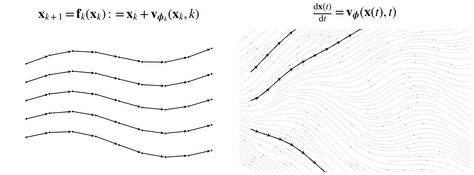
From Discrete-Time NFs to Continuous-Time NFs (Neural ODEs).
A discrete NF transports samples through a composition of \(L\) invertible maps. To obtain a meaningful continuous-depth limit, we write each layer as a small residual update: \[{\mathbf{x}}_{k+1} = {\mathbf{x}}_k+\Delta t\,{\mathbf{v}}_{\bm{\phi}}({\mathbf{x}}_k,t_k), \qquad t_k=k\Delta t, \qquad \Delta t=\frac{T}{L}.\] Here, \({\mathbf{v}}_{\bm{\phi}}\) specifies the direction in which each point is moved, while \(\Delta t\) controls the size of one layer.
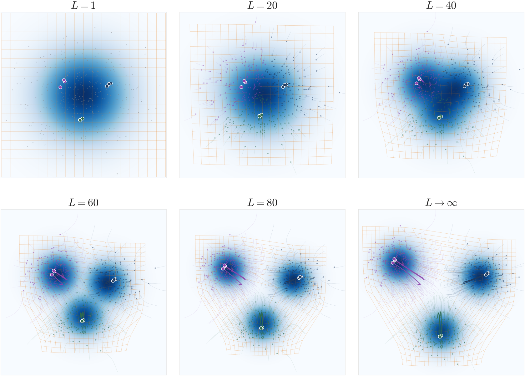
The geometric meaning of this limit is illustrated in Figure 1.5. As \(L\) increases, the same source-to-target transport is divided into more near-identity bijections. The sample trajectories are resolved more finely, and the deformation of the surrounding reference grid becomes progressively smoother.
As \(L\rightarrow\infty\) and \(\Delta t\rightarrow 0\), the discrete layer index becomes continuous time, yielding the ODE \[\frac{\mathop{}\!\mathrm{d}{\mathbf{x}}(t)}{\mathop{}\!\mathrm{d}t} = {\mathbf{v}}_{\bm{\phi}}({\mathbf{x}}(t),t).\] This continuous-depth model is known as a Neural ODE or Continuous Normalizing Flow.
Formal Setup of Neural ODEs.
A Neural ODE defines a continuous transformation through: \[\begin{align} \label{eq:neural-ode} \frac{\mathop{}\!\mathrm{d}{\mathbf{x}}(t)}{\mathop{}\!\mathrm{d}t} = {\mathbf{v}}_{\bm{\phi}}({\mathbf{x}}(t), t),\quad t\in [0,T] \end{align}\] where:
\({\mathbf{x}}(t) \in \mathbb{R}^D\) is the state at time \(t\); we sometimes write \({\mathbf{x}}_t\) for brevity;
\({\mathbf{v}}_{\bm{\phi}}({\mathbf{x}}(t), t)\) is a neural network parameterized by \(\bm{\phi}\).
Goal of NODE.
Starting from the initial condition \({\mathbf{x}}(0) \sim p_{\text{prior}}\), the ODE evolves the state continuously over time, inducing a family of marginal distributions \(p_{\bm{\phi}}({\mathbf{x}}_t, t)\) (similar to PF-ODEs!)2.
The goal is to learn the neural vector field \({\mathbf{v}}_{\bm{\phi}}\), which intuitively represents a velocity that transports points along continuous trajectories in data space. By learning this velocity, the terminal distribution at \(t=T\) matches the target distribution \(p_{\mathrm{data}}(\cdot)\). This continuous transformation unifies discrete normalizing flows and neural ODEs within a single framework.
Continuous-Time Change-of-Variables Formula.
Analogous to Equation \(\eqref{eq:nf-change-of-var}\) or Equation \(\eqref{eq:multi-nf-density}\), Chen et al. (2018) derived a continuous-time analogue of the change-of-variables formula. For the time-dependent density \(p_{\bm{\phi}}({\mathbf{x}}(t),t)\) of a process \({\mathbf{x}}(t)\) evolving under Equation \(\eqref{eq:neural-ode}\), the so-called Instantaneous Change-of-Variables Formula is \[\frac{\mathop{}\!\mathrm{d}}{\mathop{}\!\mathrm{d}t} \log p_{\bm{\phi}}({\mathbf{x}}(t),t) = -\nabla_{{\mathbf{x}}}\cdot {\mathbf{v}}_{\bm{\phi}}({\mathbf{x}}(t),t).\] Here, the derivative is taken along the ODE trajectory \({\mathbf{x}}(t)\).
Therefore, if \({\mathbf{x}}(0)\sim p_{\mathrm{prior}}\) and the ODE transports the prior from \(t=0\) to \(t=T\), integrating this identity gives \[\begin{align} \label{eq:NODE-likelihood} \log p_{\bm{\phi}}({\mathbf{x}}(T),T) = \log p_{\mathrm{prior}}({\mathbf{x}}(0)) - \int_0^T \nabla_{{\mathbf{x}}}\cdot {\mathbf{v}}_{\bm{\phi}}({\mathbf{x}}(t),t) \,\mathop{}\!\mathrm{d}t. \end{align}\] This expression provides likelihood evaluation through numerical integration, which in turn enables maximum likelihood training of the model.
Although this formula may appear unfamiliar at first, it is closely connected to the Fokker–Planck equation. In particular, it can be understood as the along-trajectory form of the continuity equation, which is the deterministic, zero-diffusion case of the Fokker–Planck equation (see Appendix B). It can also be interpreted as the continuous-time limit of the discrete change-of-variables formula in Equation \(\eqref{eq:multi-nf-density}\). We summarize the result below.
Lemma: Instantaneous Change of Variables
Let \({\mathbf{z}}(t)\) be a continuous random process with time-dependent density \(p({\mathbf{z}}(t),t)\), and suppose it evolves according to the ODE \[\begin{align*} \frac{\mathop{}\!\mathrm{d}{\mathbf{z}}(t)}{\mathop{}\!\mathrm{d}t} = \mathbf{F}({\mathbf{z}}(t),t). \end{align*}\] Assuming sufficient regularity so that the ODE flow and the evolving density are well defined, the log-density along the trajectory satisfies \[\begin{align} \label{eq:instant-change-of-var} \frac{\mathop{}\!\mathrm{d}}{\mathop{}\!\mathrm{d}t} \log p({\mathbf{z}}(t),t) = -\nabla_{{\mathbf{z}}}\cdot \mathbf{F}({\mathbf{z}}(t),t). \end{align}\]
Proof for Lemma. This follows from the continuity equation together with the chain rule. We present detailed alternative derivations in Section (Flow-Based Perspective) in Appendix D. ■
Connection to Discrete-Time Formula.
The NODE likelihood in Equation \(\eqref{eq:NODE-likelihood}\), \[\log p_{\bm{\phi}}({\mathbf{x}}(T), T) = \log p_{\text{prior}}({\mathbf{x}}(0), 0) - \int_0^T \nabla_{\mathbf{x}}\cdot {\mathbf{v}}_{\bm{\phi}}({\mathbf{x}}(t), t) \mathop{}\!\mathrm{d}t,\] can be seen as the continuous-time analogue of the discrete normalizing flow formulation in Equation \(\eqref{eq:multi-nf-density}\): \[\log p_{\bm{\phi}}({\mathbf{x}}_L) = \log p_{\text{prior}}({\mathbf{x}}_0) - \sum_{k=0}^{L-1} \log \left| \det \frac{\partial {\mathbf{f}}_k}{\partial {\mathbf{x}}_k} \right|.\] The integral mirrors the summation, and the trace operator replaces the log-determinant, as discussed in Equation \(\eqref{eq:log-det-tr}\). These parallels are further explored in the proof of the lemma.
Training NODEs.
Based on Equation \(\eqref{eq:NODE-likelihood}\), NODEs learn a parameterized velocity field \({\mathbf{v}}_{\bm{\phi}}\) such that the terminal distribution \[p_{\bm{\phi}}(\cdot, T) \approx p_{\text{data}},\] where trajectories evolve from latent variables \({\mathbf{x}}(0) \sim p_{\text{prior}}\) via the ODE flow. Training follows the MLE framework from Equation in Chapter 1 \[\mathcal{L}_{\text{NODE}}(\bm{\phi}) := \mathbb{E}_{{\mathbf{x}}\sim p_{\text{data}}} \big[\log p_{\bm{\phi}}({\mathbf{x}}, T)\big].\]
Exact Log-Likelihood Computation.
To compute \(\log p_{\bm{\phi}}(\mathbf{x}, T)\) for data point \(\mathbf{x}\), we integrate the change-of-variables formula \(\eqref{eq:NODE-likelihood}\): \[\begin{align} \log p_{\bm{\phi}}(\mathbf{x}, T) = \log p_{\text{prior}}(\mathbf{z}(0)) - \int_0^T \nabla_{\mathbf{z}} \cdot \mathbf{v}_{\bm{\phi}}(\mathbf{z}(t), t) \mathop{}\!\mathrm{d}t. \end{align}\] Here, \(\mathbf{z}(t)\) solves the ODE reversely from \(t = T\) to \(t = 0\): \[\frac{\mathop{}\!\mathrm{d}\mathbf{z}(t)}{\mathop{}\!\mathrm{d}t} = \mathbf{v}_{\bm{\phi}}(\mathbf{z}(t), t)\] with \(\mathbf{z}(T) = \mathbf{x}\). The prior term \(\log p_{\text{prior}}(\mathbf{z}(0))\) is tractable for standard distributions. This enables exact likelihood-based training and evaluation in neural ODEs.
Gradient-Based Optimization.
Maximizing \(\mathcal{L}_{\text{NODE}}\) requires backpropagation through the ODE solver. The adjoint sensitivity method (Pontryagin 2018; Chen et al. 2018) computes gradients via an auxiliary ODE with \(\mathcal{O}(1)\) memory complexity, but NODE training remains expensive due to numerical integration at each step.
Inference with NODEs.
Sampling with a trained model \({\mathbf{v}}_{\bm{\phi}^\times}\) proceeds by drawing \({\mathbf{x}}(0) \sim p_{\text{prior}}\) and integrating forward (by numerical solvers): \[{\mathbf{x}}(T) = {\mathbf{x}}(0) + \int_0^T {\mathbf{v}}_{\bm{\phi}^\times}({\mathbf{x}}(t), t) \mathop{}\!\mathrm{d}t.\] The terminal state \({\mathbf{x}}(T)\) approximates a sample from \(p_{\text{data}}\).
Moreover, we note that for any vector field \({\mathbf{F}}\), the following identity holds: \[\mathop{\mathrm{Tr}}\left(\frac{\partial {\mathbf{F}}}{\partial {\mathbf{z}}(t)} \right) = \nabla_{{\mathbf{z}}} \cdot {\mathbf{F}}.\] Hence, the divergence can be estimated efficiently using stochastic trace estimators, such as Hutchinson’s estimator (Hutchinson 1989), without explicitly constructing the full Jacobian. This makes likelihood evaluation much more practical in high-dimensional settings. However, because the trace is then estimated from random samples, the resulting numerical log-likelihood estimate is stochastic rather than an exact evaluation of the divergence.
Having seen in Figure 1.5 how many small bijections approach a continuous transport flow, we now ask a practical question:
How can we learn its velocity field without repeatedly solving an ODE during training?
This question leads naturally to Flow Matching, which learns the velocity field directly through a simulation-free regression objective and provides the flow-based perspective on diffusion models.
Flow Matching Framework
Both Score SDEs (Chapter 4) and NODEs (Section 1.1) describe generative modeling as a continuous transport process. Score SDEs formulate this transport through stochastic dynamics together with an associated PF-ODE, whereas NODEs directly parameterize a deterministic ODE. In the standard generative setting, both aim to transport a simple Gaussian prior \(p_{\mathrm{prior}}\) into the data distribution \(p_{\mathrm{data}}\).
A practical limitation of NODEs is that likelihood-based training requires repeatedly solving an ODE. The Flow Matching (FM) framework (Lipman et al. 2022, 2024; Tong et al. 2024) avoids this cost by training a neural network to predict the velocity field directly through a regression objective. ODE integration is therefore needed for generation, but not inside the training loop, making FM training simulation-free.
More generally, FM is not restricted to Gaussian-to-data transport. It considers a source distribution \(p_{\mathrm{src}}\) and a target distribution \(p_{\mathrm{tgt}}\), both assumed to be easy to sample from. Standard generative modeling is recovered as the special case \[p_{\mathrm{src}}=p_{\mathrm{prior}}, \qquad p_{\mathrm{tgt}}=p_{\mathrm{data}},\] where \(p_{\mathrm{prior}}\) is typically Gaussian.
In this section, we adopt the FM viewpoint3 Its goal is to learn a time-dependent velocity field \(\mathbf{v}_t({\mathbf{x}}_t)\) whose associated ODE transports samples along a prescribed probability path \(\{p_t\}_{t\in[0,1]}\) satisfying \[p_0=p_{\mathrm{src}}, \qquad p_1=p_{\mathrm{tgt}}.\] When \(p_{\mathrm{src}}\) is Gaussian, we refer to this setting as Gaussian Flow Matching. Thus, FM provides both a simulation-free training method for generative modeling and a general framework for learning continuous transport between arbitrary endpoint distributions.
Lesson from Score-Based Methods
We revisit the Score SDE framework (Chapter 4) using a slightly different but equivalent formulation to extract key insights that motivate the FM approach. This analysis reveals how diffusion models implicitly learn probability flows and motivates a more direct formulation.
Step 1: Defining a Conditional Path and Its Marginal Densities.
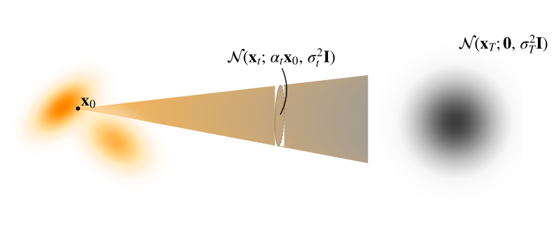
A diffusion model specifies a continuous-time family of densities \(\{p_t\}_{t \in [0,1]}\) that transports a simple prior \(p_{\text{prior}}\) (e.g., Gaussian) at \(t=1\), used as the source, to a target data distribution \(p_{\text{data}}\) at \(t=0\): \[p_1({\mathbf{x}}_1) = p_{\text{prior}}({\mathbf{x}}_1), \quad p_0({\mathbf{x}}_0) = p_{\text{data}}({\mathbf{x}}_0).\] This path is implicitly defined via the forward conditional distribution \[\begin{align} \label{eq:lesson-dm-conditional-path} p_t({\mathbf{x}}_t|{\mathbf{x}}_0) = \mathcal{N}({\mathbf{x}}_t; \alpha_t {\mathbf{x}}_0, \sigma_t^2 \mathbf{I}), \quad {\mathbf{x}}_0\sim p_{\text{data}} \end{align}\] which induces the marginal density \[p_t({\mathbf{x}}_t) := \int p_t({\mathbf{x}}_t |{\mathbf{x}}_0) p_{\text{data}}({\mathbf{x}}_0) \mathrm{d}{\mathbf{x}}_0.\] The increasing variance \(\sigma_t^2\) of the conditional Gaussian drives the evolution of \(p_t\) toward the Gaussian prior.
Step 2: Velocity Field.
The time evolution of the marginal density \(p_t\) is governed by a velocity field \({\mathbf{v}}_t : \mathbb{R}^D \to \mathbb{R}^D\), derived from the Fokker-Planck equation: \[\begin{align} \label{eq:dm-velocity} {\mathbf{v}}_t({\mathbf{x}}) := f(t){\mathbf{x}}- \frac{1}{2}g^2(t)\nabla_{{\mathbf{x}}} \log p_t({\mathbf{x}}), \end{align}\] which defines a deterministic particle flow through the PF-ODE: \[\frac{\mathop{}\!\mathrm{d}{\mathbf{x}}(t)}{\mathop{}\!\mathrm{d}t} = \underbrace{f(t){\mathbf{x}}(t) - \frac{1}{2}g^2(t)\nabla_{{\mathbf{x}}} \log p_t\big({\mathbf{x}}(t)\big)}_{{\mathbf{v}}_t({\mathbf{x}}(t))}.\] This ODE transports an initial random variable \({\mathbf{x}}(0) \sim p_{\text{data}}\) forward in time or \({\mathbf{x}}(1) \sim p_{\text{prior}}\) backward in time, such that the evolving marginal density of \({\mathbf{x}}(t)\) matches \(p_t\) at every \(t \in [0,1]\) (see “Underlying Rule” below).
The scalar functions \(f(t)\) and \(g(t)\) are determined by the coefficients of the associated forward SDE, or equivalently the Gaussian kernel parameters \(\alpha_t\) and \(\sigma_t\) defined in the conditional path (see Lemma in Chapter 4 (Forward Perturbation Kernel ⟺ Linear SDE)).
Step 3: Learning via the Conditional Strategy.
The PF-ODE velocity in Equation \(\eqref{eq:dm-velocity}\) depends on the marginal score \(\nabla_{{\mathbf{x}}_t}\log p_t({\mathbf{x}}_t)\), which is generally unknown. Score-based methods therefore learn this score using a neural network \({\mathbf{s}}_{\bm{\phi}}({\mathbf{x}}_t,t)\) through the ideal score-matching objective \[\mathcal{L}_{\text{SM}}(\bm{\phi}) = \mathbb{E}_{t\sim\mathcal{U}[0,1],\,{\mathbf{x}}_t\sim p_t} \left[ \left\| {\mathbf{s}}_{\bm{\phi}}({\mathbf{x}}_t,t) - \nabla_{{\mathbf{x}}_t}\log p_t({\mathbf{x}}_t) \right\|^2 \right].\] Once the score is learned, the PF-ODE velocity is obtained from it as \[{\mathbf{v}}_t({\mathbf{x}}_t) = f(t){\mathbf{x}}_t - \frac{1}{2}g^2(t) \nabla_{{\mathbf{x}}_t}\log p_t({\mathbf{x}}_t),\] with \({\mathbf{s}}_{\bm{\phi}^\times}({\mathbf{x}},t) \approx \nabla_{{\mathbf{x}}_t}\log p_t({\mathbf{x}})\)
The difficulty is that the marginal score itself is inaccessible when computing the regression target. As in Chapter 3, we overcome this using the conditioning trick. The conditional distribution \(p_t({\mathbf{x}}_t|{\mathbf{x}}_0)\) is tractable, and its conditional score satisfies \[\begin{align} \label{eq:marginal-oracle-score} \nabla_{{\mathbf{x}}_t}\log p_t({\mathbf{x}}_t) = \mathbb{E}_{{\mathbf{x}}_0\sim p(\cdot|{\mathbf{x}}_t)} \left[ \nabla_{{\mathbf{x}}_t}\log p_t({\mathbf{x}}_t|{\mathbf{x}}_0) \right]. \end{align}\] This motivates the denoising score matching objective \[\mathcal{L}_{\text{DSM}}(\bm{\phi}) := \mathbb{E}_{t,\,{\mathbf{x}}_0\sim p_{\mathrm{data}},\, {\mathbf{x}}_t\sim p_t(\cdot|{\mathbf{x}}_0)} \left[ \left\| {\mathbf{s}}_{\bm{\phi}}({\mathbf{x}}_t,t) - \nabla_{{\mathbf{x}}_t}\log p_t({\mathbf{x}}_t|{\mathbf{x}}_0) \right\|^2 \right].\] As shown in Theorem in Chapter 3 (Equivalence of L_SM and L_DSM), \(\mathcal{L}_{\text{SM}}\) and \(\mathcal{L}_{\text{DSM}}\) differ only by a constant independent of \(\bm{\phi}\) and therefore have the same population minimizer: \[{\mathbf{s}}^*({\mathbf{x}}_t,t) = \mathbb{E}_{{\mathbf{x}}_0\sim p(\cdot|{\mathbf{x}}_t)} \left[ \nabla_{{\mathbf{x}}_t}\log p_t({\mathbf{x}}_t|{\mathbf{x}}_0) \right] = \nabla_{{\mathbf{x}}_t}\log p_t({\mathbf{x}}_t).\]
Importantly, the same conditioning principle can also be expressed directly at the level of the PF-ODE velocity. Define the conditional velocity \[{\mathbf{v}}_t({\mathbf{x}}_t|{\mathbf{x}}_0) := f(t){\mathbf{x}}_t - \frac{1}{2}g^2(t) \nabla_{{\mathbf{x}}_t}\log p_t({\mathbf{x}}_t|{\mathbf{x}}_0).\] Using Equation \(\eqref{eq:marginal-oracle-score}\), we immediately obtain \[{\mathbf{v}}_t({\mathbf{x}}_t) = \mathbb{E}_{{\mathbf{x}}_0\sim p(\cdot|{\mathbf{x}}_t)} \left[ {\mathbf{v}}_t({\mathbf{x}}_t|{\mathbf{x}}_0) \right].\] Thus, score-based diffusion learns the score through tractable conditional targets and then uses it to construct the PF-ODE velocity. Flow Matching will apply the same conditional-to-marginal principle directly to the velocity field.

Underlying Rule: The Fokker–Planck Equation.
The marginal density \(p_t\) evolves according to the Fokker–Planck equation:
\[\begin{align*} \frac{\partial p_t({\mathbf{x}})}{\partial t} + \nabla \cdot \Bigg( \underbrace{\left(f(t){\mathbf{x}}- \frac{1}{2}g^2(t) \nabla_{\mathbf{x}}\log p_t({\mathbf{x}})\right)}_{{\mathbf{v}}_t({\mathbf{x}})} p_t({\mathbf{x}}) \Bigg) = 0. \end{align*}\]
This PDE ensures that the density given by the PF-ODE matches the marginal distribution of the forward SDE. To see this, recall the flow map \({\bm{\Psi}}_{s \to t}({\mathbf{x}}_s)\) of the PF-ODE as defined in Equation in Chapter 4, which carries an initial state \({\mathbf{x}}_s\) at time \(s\) directly to its state at \(t\). Running the PF-ODE backward from \(t=1\) to \(t=0\), starting with \({\mathbf{x}}_1 \sim p_{\mathrm{prior}}\), we obtain time-dependent densities through the pushforward formula: \[\begin{align} \label{eq:pushforward-ode} p_t^{\mathrm{rev}}({\mathbf{x}}) = \int \delta \left({\mathbf{x}}- {\bm{\Psi}}_{1 \to t}({\mathbf{x}}_1)\right) p_{\mathrm{prior}}({\mathbf{x}}_1) \mathrm{d}{\mathbf{x}}_1. \end{align}\]
The Fokker–Planck equation ensures that the induced density path coincides with the same evolving density: \[\begin{align} \label{eq:p_t-fwd-rev} p_t^{\mathrm{rev}} = p_t. \end{align}\] In particular, this implies \(p_0^{\mathrm{rev}} = p_0 = p_{\text{data}}\), thereby recovering the data distribution at time \(t=0\). Since the ODE solution map is bidirectional, we can similarly consider initializing at \({\mathbf{x}}_0 \sim p_{\text{data}}\) and solving the ODE forward in time, enabling a parallel analysis.
Flow Matching Framework
The analysis in Section 1.2.1 reveals that diffusion models succeed by learning a velocity field, specifically, the score, that transports between distributions while satisfying boundary conditions. The design of the Gaussian conditional path in Equation \(\eqref{eq:lesson-dm-conditional-path}\), with increasing variance \(\sigma_t^2\), implicitly anchors one endpoint to a Gaussian prior while allowing the conditional density to be defined over the entire space, enabling score-based gradient computation.
In this subsection, we introduce the FM framework, which builds on this insight (the same illustration in Figure 1.7 also applies to the FM framework) and extends it to learning continuous flows that transport samples between two arbitrary distributions, \(p_{\text{src}}\) and \(p_{\text{tgt}}\).
Step 1: Defining a Conditional Path and Its Marginal Densities.
Consider arbitrary source and target probability distributions \(p_{\mathrm{src}}\) and \(p_{\mathrm{tgt}}\) on \(\mathbb{R}^D\). We set4 \[\begin{align} \label{eq:marginal-endpoint} p_0(\mathbf{x}) = p_{\mathrm{src}}(\mathbf{x}), \quad p_1(\mathbf{x}) = p_{\mathrm{tgt}}(\mathbf{x}). \end{align}\]
FM implicitly defines a continuous family of intermediate densities \(\{ p_t \}_{t \in [0,1]}\) interpolating between these endpoints. Each marginal \(p_t\) is expressed via a latent variable \(\mathbf{z}\) drawn from a known distribution \(\pi(\mathbf{z})\) and a conditional distribution \(p_t(\mathbf{x}_t | \mathbf{z})\): \[\begin{equation} \label{eq:p_t} p_t(\mathbf{x}_t) = \int p_t(\mathbf{x}_t | \mathbf{z}) \pi(\mathbf{z}) \mathop{}\!\mathrm{d}\mathbf{z}, \end{equation}\] with \((\pi(\mathbf{z}), \{p_t(\cdot|\mathbf{z})\})\) chosen to satisfy the boundary conditions in Equation \(\eqref{eq:marginal-endpoint}\).
We remark that, in general, the marginal densities \(p_t\) are not tractable, since they require integrating over \(\pi(\mathbf{z})\), and both \(\pi(\mathbf{z})\) and the conditional distributions \(p_t(\mathbf{x}_t|\mathbf{z})\) can be complex. Nonetheless, conditioning on the latent \(\mathbf{z}\) grants FM the flexibility to model a broad class of interpolation paths beyond those discussed in Section 1.2.1. Common choices for \(\mathbf{z}\) include:
Two-sided conditioning: \(\mathbf{z} = (\mathbf{x}_0, \mathbf{x}_1) \sim p_{\text{src}}(\mathbf{x}_0) p_{\text{tgt}}(\mathbf{x}_1)\), where \(\pi\) couples source and target distributions. This allows FM to define transport between arbitrary distributions.
One-sided conditioning: \(\mathbf{z} = \mathbf{x}_0\) or \(\mathbf{z} = \mathbf{x}_1\). It especially recovers diffusion-like setups when the source distribution is chosen to be Gaussian.
In all cases, the conditional path \(p_t(\mathbf{x}_t|\mathbf{z})\) should be efficiently sampleable, and the corresponding conditional velocity should be tractable. In the probability-path-first constructions below, we further use conditional distributions with tractable closed-form expressions. We present specific constructions in Section 1.3.2, with illustrations in Figure 1.9.
Step 2: Velocity Field.
A probability path \(\{p_t\}_{t\in[0,1]}\) specifies how the distribution should evolve over time, but it does not generally specify how individual samples should move. In other words, the same sequence of marginal densities can be realized by different velocity fields5.
The goal of FM is therefore to find a velocity field \(\mathbf{v}_t(\mathbf{x})\) whose induced ODE \[\frac{\mathop{}\!\mathrm{d}\mathbf{x}(t)}{\mathop{}\!\mathrm{d}t} = \mathbf{v}_t(\mathbf{x}(t)), \qquad t\in[0,1],\] produces marginal distributions that match the prescribed \(p_t\) at every time \(t\). When this holds, the ODE can transport samples forward from \(\mathbf{x}(0)\sim p_{\text{src}}\) to \(p_{\text{tgt}}\), or backward from \(\mathbf{x}(1)\sim p_{\text{tgt}}\) to \(p_{\text{src}}\) (see Section 1.2.4 for a more formal discussion).
This requirement is captured by the continuity equation6:
\[\begin{equation} \label{eq:continuity_eq} \frac{\partial p_t(\mathbf{x})}{\partial t} + \nabla\cdot \bigl( \mathbf{v}_t(\mathbf{x})p_t(\mathbf{x}) \bigr) = 0. \end{equation}\]
Any velocity field \(\mathbf{v}_t\) satisfying Equation \(\eqref{eq:continuity_eq}\), together with the initial condition \(p_0=p_{\mathrm{src}}\), generates an ODE whose evolving marginals follow the prescribed path \(\{p_t\}\), under suitable regularity conditions. Thus, solving the ODE provides a sample-wise transport between \(p_{\mathrm{src}}\) and \(p_{\mathrm{tgt}}\) while matching the intermediate distributions.
Importantly, the continuity equation constrains the evolution of probability density, but generally does not uniquely determine the velocity field. Different sample trajectories can therefore produce exactly the same marginal density evolution. For example, on regions where \(p_t>0\), if \(\mathbf{v}_t\) satisfies Equation \(\eqref{eq:continuity_eq}\), then \[\mathbf{v}_t + \frac{1}{p_t}\tilde{\mathbf{v}}_t\] also satisfies it for any sufficiently regular divergence-free field \(\tilde{\mathbf{v}}_t\) with \(\nabla\cdot\tilde{\mathbf{v}}_t=0\).
FM therefore seeks a velocity field that realizes the prescribed probability path. For general source and target distributions, neither the marginal density \(p_t\) nor such a velocity field is usually available in closed form. This motivates the conditional construction introduced next, where tractable conditional paths and velocities are used to learn a valid marginal velocity field.
As a concrete illustration, in Section 1.3.1 we consider a Gaussian-to-Gaussian path together with a particular affine flow map, for which the corresponding velocity field can be computed explicitly.
Step 3: Learning via the Conditional Strategy.
Once a probability path and a corresponding marginal velocity field \({\mathbf{v}}_t\) have been chosen, FM learns this velocity field directly using a neural network \({\mathbf{v}}_{\bm{\phi}}\). The ideal FM objective is \[\mathcal{L}_{\mathrm{FM}}(\bm{\phi}) = \mathbb{E}_{t,\,{\mathbf{x}}_t\sim p_t} \left[ \left\| {\mathbf{v}}_{\bm{\phi}}({\mathbf{x}}_t,t) - {\mathbf{v}}_t({\mathbf{x}}_t) \right\|^2 \right].\] We refer to this neural network parameterization as \({\mathbf{v}}\)-prediction (velocity prediction), since the network directly predicts the drift of the ODE. This differs from the score-based construction in Section 1.2.1, where the score is learned first and then used to construct the PF-ODE velocity.
The difficulty is that the marginal velocity \({\mathbf{v}}_t({\mathbf{x}}_t)\) is generally intractable. As in denoising score matching, we overcome this using a conditioning strategy. We introduce a latent variable \({\mathbf{z}}\sim\pi({\mathbf{z}})\) and construct a tractable conditional probability path \(p_t({\mathbf{x}}_t|{\mathbf{z}})\) together with a corresponding conditional velocity field \({\mathbf{v}}_t({\mathbf{x}}_t|{\mathbf{z}})\).
If each conditional velocity field generates its corresponding conditional probability path, then marginalizing over \({\mathbf{z}}\) gives a valid marginal velocity field: \[\begin{align} \label{eq:marginal-oracle-velocity} {\mathbf{v}}_t({\mathbf{x}}_t) := \mathbb{E}_{{\mathbf{z}}\sim p(\cdot|{\mathbf{x}}_t)} \left[ {\mathbf{v}}_t({\mathbf{x}}_t|{\mathbf{z}}) \right]. \end{align}\] Thus, the generally intractable marginal velocity is the conditional average of tractable conditional velocities. This is directly analogous to the conditional-score identity in Equation \(\eqref{eq:marginal-oracle-score}\).
This observation leads to the conditional flow matching (CFM) objective:
\[\begin{align} \label{eq:fm-cfm} \mathcal{L}_{\mathrm{CFM}}(\bm{\phi}) := \mathbb{E}_{t,\,{\mathbf{z}}\sim\pi({\mathbf{z}}),\, {\mathbf{x}}_t\sim{\color{orange}p_t(\cdot|{\mathbf{z}})}} \left[ \left\| {\mathbf{v}}_{\bm{\phi}}({\mathbf{x}}_t,t) - {\color{orange}{\mathbf{v}}_t({\mathbf{x}}_t|{\mathbf{z}})} \right\|^2 \right]. \end{align}\]
Here, \({\mathbf{z}}\) is used to construct the training sample \({\mathbf{x}}_t\) and the conditional regression target \({\mathbf{v}}_t({\mathbf{x}}_t|{\mathbf{z}})\); it is not an additional input to the neural network \({\mathbf{v}}_{\bm{\phi}}({\mathbf{x}}_t,t)\). Importantly, the two objectives differ only by a constant \(C\leq0\) independent of \(\bm{\phi}\): \[\mathcal{L}_{\mathrm{FM}}(\bm{\phi}) = \mathcal{L}_{\mathrm{CFM}}(\bm{\phi}) + C.\] They therefore have the same population minimizer, \[\begin{align} \label{eq:minimum_velocity} {\mathbf{v}}^*({\mathbf{x}}_t,t) = {\mathbf{v}}_t({\mathbf{x}}_t). \end{align}\] In other words, although each training example uses a conditional velocity \({\mathbf{v}}_t({\mathbf{x}}_t|{\mathbf{z}})\) as its target, averaging over these examples recovers the desired marginal velocity field.
For CFM to provide tractable, simulation-free training, two practical conditions are needed:
we can easily sample \({\mathbf{x}}_t\sim p_t(\cdot|{\mathbf{z}})\) without solving an ODE;
the conditional velocity \({\mathbf{v}}_t({\mathbf{x}}_t|{\mathbf{z}})\) has a tractable expression that can be used as the regression target.
We provide concrete constructions satisfying these conditions in Section 1.3.2. Thus, just as denoising score matching learns an intractable marginal score through tractable conditional scores, Flow Matching learns an intractable marginal velocity through tractable conditional-velocity targets.
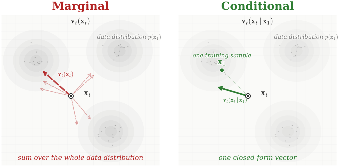
We summarize the above discussion as follows:
Theorem: Equivalence of \(\mathcal{L}_{\mathrm{FM}}\) and \(\mathcal{L}_{\mathrm{CFM}}\)
The following holds: \[\begin{align*} \mathcal{L}_{\mathrm{FM}}(\bm{\phi}) = \mathcal{L}_{\mathrm{CFM}}(\bm{\phi}) + C, \end{align*}\] where \(C\) is a constant independent of the parameter \(\bm{\phi}\). Furthermore, the minimizer \({\mathbf{v}}^*\) of both losses satisfies \[{\mathbf{v}}^*({\mathbf{x}}_t, t) = {\mathbf{v}}_t({\mathbf{x}}_t), \quad \text{for almost every } {\mathbf{x}}_t \sim p_t,\] where \({\mathbf{v}}_t({\mathbf{x}}_t)\) is defined in Equation \(\eqref{eq:marginal-oracle-velocity}\).
Proof for Theorem. The argument and derivation of the minimizer follows exactly the same reasoning as in the score matching case of Proposition in Chapter 4 (Minimizer of DSM). ■
This marks the third instance where the conditioning trick yields a tractable training objective, as illustrated in Figure 1.8. Notably, the variational, score based, and flow based approaches all reflect the same underlying principle.
Remark. Taking \(\pi = p_{\mathrm{data}}\), we can apply Bayes’ rule: \[p({\mathbf{x}}_0|{\mathbf{x}}_t) = \frac{p_t({\mathbf{x}}_t|{\mathbf{x}}_0) p_{\mathrm{data}}({\mathbf{x}}_0)}{p_t({\mathbf{x}}_t)},\] a similar decomposition of Equation \(\eqref{eq:marginal-oracle-velocity}\) appears in score-based models: \[\begin{align*} \nabla_{{\mathbf{x}}_t} \log p_t({\mathbf{x}}_t) &= \mathbb{E}_{{\mathbf{x}}_0 \sim p(\cdot|{\mathbf{x}}_t)} \left[ \nabla_{{\mathbf{x}}_t} \log p_t({\mathbf{x}}_t|{\mathbf{x}}_0) \right] \\ &= \mathbb{E}_{{\mathbf{x}}_0 \sim p_{\text{data}}} \left[ \nabla_{{\mathbf{x}}_t} \log p_t({\mathbf{x}}_t|{\mathbf{x}}_0) \cdot \frac{p_t({\mathbf{x}}_t|{\mathbf{x}}_0)}{p_t({\mathbf{x}}_t)} \right], \end{align*}\] which mirrors the marginalization strategy in Equation \(\eqref{eq:marginal-oracle-velocity}\).
As in Section 1.2.1, where the conditional density \(p_t({\mathbf{x}}_t|{\mathbf{z}})\) and conditional velocity field \({\mathbf{v}}_t({\mathbf{x}}_t|{\mathbf{z}})\) must be explicitly specified, with \(p_t({\mathbf{x}}_t|{\mathbf{x}}_0) = \mathcal{N}({\mathbf{x}}_t; \alpha_t {\mathbf{x}}_0, \sigma_t^2 {\mathbf{I}})\) and \({\mathbf{v}}_t({\mathbf{x}}_t|{\mathbf{x}}_0) = f(t){\mathbf{x}}_t - \frac{1}{2}g^2(t)\nabla_{{\mathbf{x}}_t} \log p_t({\mathbf{x}}_t|{\mathbf{x}}_0)\), the general conditional flow matching framework also requires these two components. However, we have not yet construct the conditional density \(p_t({\mathbf{x}}_t|{\mathbf{z}})\) or the conditional velocity field \({\mathbf{v}}_t({\mathbf{x}}_t|{\mathbf{z}})\) in this general case. In Section 1.3, we introduce several common instantiations of these components.
Comparison of Diffusion Models, General Flow Matching, and NODEs
Comparison of Diffusion Models and General Flow Matching.
The insight from Section 1.2.1 leads to an extended FM framework that retains the same underlying principles. To highlight their similarities, we summarize them in Table 1.1.
| Aspect | (Score-Based) Diffusion Model | General FM |
|---|---|---|
| Source dist. \(p_{\mathrm{src}}\) | Gaussian prior | Any |
| Target dist. \(p_{\mathrm{tgt}}\) | Data distribution | Any |
| Latent dist. \(\pi({\mathbf{z}})\) | \(p_{\text{data}}\) | See Section 1.3.2 |
| Cond. dist. \(p_t({\mathbf{x}}_t|{\mathbf{z}})\) | \(\mathcal{N}({\mathbf{x}}_t;\alpha_t{\mathbf{x}}_0,\sigma_t^2{\mathbf{I}})\) | See Section 1.3.2 |
| Marginal dist. \(p_t({\mathbf{x}}_t)\) | \(\int p_t({\mathbf{x}}_t|{\mathbf{x}}_0) p_{\mathrm{data}}({\mathbf{x}}_0) \mathop{}\!\mathrm{d}{\mathbf{x}}_0\) | \(\int p_t({\mathbf{x}}_t|{\mathbf{z}}) \pi({\mathbf{z}}) \mathop{}\!\mathrm{d}{\mathbf{z}}\) |
| Cond. velocity \({\mathbf{v}}_t({\mathbf{x}}|{\mathbf{z}})\) | \(f(t) {\mathbf{x}}- \frac{1}{2} g^2(t) \nabla \log p_t({\mathbf{x}}|{\mathbf{x}}_0)\) | See Section 1.3.2 |
| Marginal velocity \({\mathbf{v}}_t({\mathbf{x}})\) | \(f(t) {\mathbf{x}}- \frac{1}{2} g^2(t) \nabla \log p_t({\mathbf{x}})\) | See Equation \(\eqref{eq:marginal-oracle-velocity}\) |
| Learning objective | \(\mathcal{L}_{\text{SM}}=\mathcal{L}_{\text{DSM}}+C\) | \(\mathcal{L}_{\mathrm{FM}}=\mathcal{L}_{\mathrm{CFM}}+C\) |
| Underlying Rule | Fokker-Planck / Continuity Equation | |
We remark that, assuming the Gaussian schedule satisfies the diffusion-SDE compatibility condition in Lemma in Chapter 4 (Forward Perturbation Kernel ⟺ Linear SDE), Gaussian FM is essentially equivalent to the corresponding diffusion formulation (see more in Chapter 6); we therefore do not differentiate between them unless explicitly stated.
Connection to NODEs.
FM can be viewed as a simulation-free alternative to NODEs, introduced in Section 1.1.2. While CNFs require solving ODEs during maximum likelihood training, which is computationally intensive, FM bypasses this by directly regressing a prescribed velocity field through a simple regression loss. The key insight is that when the marginal density path connecting the source and target distributions is fixed, exact simulation during training becomes unnecessary.
(Optional) Underlying Rules
Continuity Equation: Mass Conservation Criterion.
Similar to the PF-ODE and Fokker–Planck analysis in Section 1.2.1, we now present a criterion for verifying whether the density path induced by an ODE flow aligns with a prescribed path \(\{p_t\}_{t \in [0,1]}\).
Consider the ODE describing the flow of particles under a time-dependent velocity field \({\mathbf{v}}_t\): \[\frac{\mathop{}\!\mathrm{d}{\mathbf{x}}(t)}{\mathop{}\!\mathrm{d}t} = {\mathbf{v}}_t\left({\mathbf{x}}(t)\right).\] As in Equation \(\eqref{eq:pushforward-ode}\), this ODE defines a flow map \(\bm{\Psi}_{s\to t}({\mathbf{x}}_0)\) for any \(s,t \in [0,1]\), which in particular transports an initial point \({\mathbf{x}}_0 \sim p_{\mathrm{src}}\) at time \(0\) to its state at time \(t\). The induced distribution at time \(t\) is given by the pushforward \[\begin{align} \label{eq:ode-pushforward} p_t^{\mathrm{fwd}}({\mathbf{x}}) = \int \delta \left({\mathbf{x}}- \bm{\Psi}_{0\to t}({\mathbf{x}}_0)\right) p_{\mathrm{src}}({\mathbf{x}}_0) \mathrm{d}{\mathbf{x}}_0=: \bm{\Psi}_{0\to t}\# p_{\mathrm{src}}, \end{align}\] so that \(\bm{\Psi}_{0\to t}({\mathbf{x}}_0) \sim p_t^{\mathrm{fwd}}\) whenever \({\mathbf{x}}_0 \sim p_{\mathrm{src}}\). Similarly, one can transport backward from \({\mathbf{x}}_1 \sim p_{\mathrm{tgt}}\) to \(p_{\mathrm{src}}\) via \(\bm{\Psi}_{1\to 0}({\mathbf{x}}_1)\).
Suppose we are given a prescribed density path \(\{p_t\}_{t \in [0,1]}\), and we construct a velocity field \(\{{\mathbf{v}}_t\}_{t \in [0,1]}\) to define a particle flow. This naturally raises the question:
Under what conditions does the flow-induced density \(p_t^{\mathrm{fwd}}\) exactly match the target density \(p_t\) for all \(t \in [0,1]\)?
Once the two density evolutions align, we can leverage the ODE flow to flexibly transport samples between \(p_{\mathrm{src}}\) and \(p_{\mathrm{tgt}}\) by solving the ODE.
As in Equation \(\eqref{eq:p_t-fwd-rev}\), a principled way to verify this alignment is via the continuity equation, which captures the conservation of mass in time-evolving densities:
Theorem: Mass Conservation Criterion
The flow-induced density \(p_t^{\mathrm{fwd}}\) equals the prescribed path \(p_t\) for all \(t \in [0,1]\); i.e., \[p_t^{\mathrm{fwd}} = p_t, \quad \text{for all } t \in [0,1],\] if and only if the pair \((p_t, {\mathbf{v}}_t)\) satisfies the continuity equation: \[\partial_t p_t({\mathbf{x}}) + \nabla_{\mathbf{x}}\cdot (p_t({\mathbf{x}}) {\mathbf{v}}_t({\mathbf{x}})) = 0,\] for all \(t\in[0,1]\) and \({\mathbf{x}}\).
Proof for Theorem. A conceptual derivation is provided in Section (Mass Conservation Criterion) in Appendix D, while a more rigorous treatment can be found in (Villani et al. 2008) (see “Mass Conservation Formula”). ■
From Conditional to Marginal Paths.
As seen in Section 1.2.2, we begin by defining a conditional probability path \(p_t(\cdot| {\mathbf{z}})\) and a corresponding conditional velocity field \({\mathbf{v}}_t(\cdot| {\mathbf{z}})\). We then construct the marginal velocity field via: \[{\mathbf{v}}_t({\mathbf{x}}) = \int {\mathbf{v}}_t({\mathbf{x}}| {\mathbf{z}}) \frac{p_t({\mathbf{x}}| {\mathbf{z}}) \pi({\mathbf{z}})}{p_t({\mathbf{x}})} \mathop{}\!\mathrm{d}{\mathbf{z}},\] as in Equation \(\eqref{eq:marginal-oracle-velocity}\). However, we still need to ensure that the resulting marginal velocity \({\mathbf{v}}_t\) induces an ODE flow whose density path aligns with the prescribed \(p_t\). Fortunately, this verification can be done entirely at the conditional level: if each conditional velocity field \({\mathbf{v}}_t(\cdot| {\mathbf{z}})\) induces the conditional density path \(p_t(\cdot| {\mathbf{z}})\), then the resulting marginal velocity \({\mathbf{v}}_t\) also induces the correct marginal path. Formally, we state the result below and provide the complete derivation in one place to show explicitly how the marginal velocity field takes this form:
Proposition: Marginal VF Generates Given Marginal Density
If the conditional velocity fields \({\mathbf{v}}_t(\cdot|{\mathbf{z}})\) induce conditional density paths that match \(p_t(\cdot|{\mathbf{z}})\) (starting from \(p_0(\cdot|{\mathbf{z}})\)), then the marginal velocity field \({\mathbf{v}}_t(\cdot)\) defined in Equation \(\eqref{eq:marginal-oracle-velocity}\) induces a marginal density path that aligns with \(p_t(\cdot)\), starting from \(p_0(\cdot)\).
Proof for Proposition. This result follows by verifying that the pair \((p_t, {\mathbf{v}}_t)\) satisfies the Continuity Equation. We present the argument in a converse manner to provide intuition for why the marginalized velocity field takes the form in Equation \(\eqref{eq:marginal-oracle-velocity}\). Since the conditional velocity fields \({\mathbf{v}}_t(\cdot|{\mathbf{z}})\) induce density paths matching the conditional densities \(p_t(\cdot|{\mathbf{z}})\) for \({\mathbf{z}}\sim \pi\), the continuity equation holds for each conditional pair: \[\begin{align} \label{eq:continuity_conditional_pt} \frac{\mathop{}\!\mathrm{d}}{\mathop{}\!\mathrm{d}t} p_t({\mathbf{x}}|{\mathbf{z}}) =- \nabla_{\mathbf{x}}\cdot \big({\mathbf{v}}_t({\mathbf{x}}|{\mathbf{z}}) p_t({\mathbf{x}}|{\mathbf{z}})\big). \end{align}\] We aim to find a velocity field \({\color{orange}{\mathbf{v}}_t(\cdot)}\) whose induced densities align with the marginal density \(p_t\), i.e., satisfy \[\begin{align} \label{eq:p_t_continuity} \frac{\mathop{}\!\mathrm{d}}{\mathop{}\!\mathrm{d}t} p_t({\mathbf{x}}) =- \nabla_{\mathbf{x}}\cdot \big({\color{orange}{\mathbf{v}}_t({\mathbf{x}})} p_t({\mathbf{x}})\big). \end{align}\] Starting from the definition of \(p_t\) in Equation \(\eqref{eq:p_t}\), \[\begin{align*} \frac{\mathop{}\!\mathrm{d}}{\mathop{}\!\mathrm{d}t} p_t({\mathbf{x}}) &=\int \frac{\mathop{}\!\mathrm{d}}{\mathop{}\!\mathrm{d}t} p_t({\mathbf{x}}_t|{\mathbf{z}})\pi({\mathbf{z}})\mathop{}\!\mathrm{d}{\mathbf{z}}\nonumber\\ &= - \int \nabla_{\mathbf{x}}\cdot\Big( {\mathbf{v}}_t({\mathbf{x}}|{\mathbf{z}}) p_t({\mathbf{x}}| {\mathbf{z}}) \Big)\pi({\mathbf{z}}) \mathop{}\!\mathrm{d}{\mathbf{z}}\quad \nonumber \\ &= -\nabla_{\mathbf{x}}\cdot \Big( \int {\mathbf{v}}_t({\mathbf{x}}|{\mathbf{z}}) p_t({\mathbf{x}}| {\mathbf{z}}) \pi({\mathbf{z}}) \mathop{}\!\mathrm{d}{\mathbf{z}}\Big), \nonumber \end{align*}\] where the second equality follows by applying Equation \(\eqref{eq:continuity_conditional_pt}\). Comparing this with the right-hand side of Equation \(\eqref{eq:p_t_continuity}\) shows that, up to a divergence-free term, \[{\color{orange}{\mathbf{v}}_t({\mathbf{x}})} p_t({\mathbf{x}}) = \int {\mathbf{v}}_t({\mathbf{x}}|{\mathbf{z}}) p_t({\mathbf{x}}|{\mathbf{z}}) \pi({\mathbf{z}}) \mathop{}\!\mathrm{d}{\mathbf{z}}.\] Therefore, we can define \[{\color{orange}{\mathbf{v}}_t({\mathbf{x}})} := \int {\mathbf{v}}_t({\mathbf{x}}|{\mathbf{z}}) \frac{p_t({\mathbf{x}}|{\mathbf{z}})}{p_t({\mathbf{x}})} \pi({\mathbf{z}}) \mathop{}\!\mathrm{d}{\mathbf{z}},\] which is precisely the form in Equation \(\eqref{eq:marginal-oracle-velocity}\). The proof of this theorem essentially follows the reverse of this argument. ■
This connection allows us to reduce the construction of the potentially intractable marginal velocity field to defining simpler conditional fields \({\mathbf{v}}_t(\cdot| {\mathbf{z}})\), which are easier to work with by construction.
Constructing Probability Paths and Velocities Between Distributions
The essence of flow matching lies in the gradual transformation of a source distribution into a target. To direct this transformation, two key elements are needed: the probability path \(p_{t}\), which provides a snapshot of the evolving distribution at each time \(t\), and the velocity field \({\mathbf{v}}_{t}\), which describes how individual particles move along the path. These two objects are not independent; they are linked through the continuity equation, which ensures that particle dynamics are consistent with the evolution of the distribution. Thus, the learning task reduces to finding a velocity field \({\mathbf{v}}_t\) that faithfully drives the process. The difficulty, however, is that for general and complex distributions, the true marginal velocity \({\mathbf{v}}_t\) is unknown, leaving us with an intractable target that cannot be accessed directly.
The core idea of Conditional Flow Matching is to address the intractability of the true marginal velocity by constructing an artificial but tractable process. To do this, we introduce a conditioning variable \({\mathbf{z}}\) and design either a conditional velocity \({\mathbf{v}}_t({\mathbf{x}}_t|{\mathbf{z}})\) and/or a conditional path \(p_t({\mathbf{x}}_t|{\mathbf{z}})\), which are deliberately chosen to be simple.
Because these conditional objects are known in closed form, they serve as surrogate targets that the model can regress against. This leads to a valid training loss \(\mathcal{L}_{\mathrm{CFM}}\), provided two practical requirements are met: (i) we can sample efficiently from \(p_t(\cdot|{\mathbf{z}})\), and (ii) the corresponding velocity \({\mathbf{v}}_t(\cdot|{\mathbf{z}})\) admits a closed-form expression.
How should we design a well behaved conditional process? For inspiration, we turn to the one case that is fully understood: the Gaussian to Gaussian bridge (Section 1.3.1). This example highlights two natural design strategies: adopt a Gaussian probability path at each time \(t\), or prescribe an affine velocity field, both of which are analytically tractable.
Guided by this insight, we extend to general endpoint distributions using two complementary construction views (see also Section (Continuous-Time Limit: Continuity Equation) in Appendix B). These correspond to the classical Eulerian and Lagrangian descriptions of transport:
Conditional Probability-Path First (Eulerian View). We begin with the conditional density path \(p_t(\cdot|{\mathbf{z}})\) and seek a conditional velocity field \({\mathbf{v}}_t(\cdot|{\mathbf{z}})\) satisfying the continuity equation. Since a density path alone generally does not determine a unique velocity, this construction also requires choosing a particular compatible velocity field.
Conditional Flow First (Lagrangian View). We instead specify how individual particles move through a conditional flow map \({\bm{\Psi}}_{0\to t}(\cdot|{\mathbf{z}})\). The induced density is obtained by pushforward, and, when the flow map is invertible, the corresponding Eulerian velocity field is \[{\mathbf{v}}_t = \partial_t{\bm{\Psi}}_{0\to t} \circ {\bm{\Psi}}_{0\to t}^{-1}.\]
In Section 1.3.2, we detail the first approach, which shows its close analogy to diffusion model construction discussed in Section 1.2.1, while in Section 1.3.3 we present the second. Together, these perspectives provide a practical framework for defining \(p_t({\mathbf{x}}_t| {\mathbf{z}})\) and \({\mathbf{v}}_t({\mathbf{x}}_t| {\mathbf{z}})\), enabling simulation-free training and the construction of flows between arbitrary source and target distributions.
A Key Special Case: Marginal \(p_t({\mathbf{x}}_t)\) and Velocity \({\mathbf{v}}_t({\mathbf{x}}_t)\) in the Gaussian-to-Gaussian Bridge
We begin with the Gaussian–endpoint case, where we can compute the marginal density \(p_t({\mathbf{x}}_t)\) and velocity field \({\mathbf{v}}_t({\mathbf{x}}_t)\) analytically. This serves as a template for the general construction of the conditional density \(p_t({\mathbf{x}}_t |{\mathbf{z}}_t)\) and velocity field \({\mathbf{v}}_t({\mathbf{x}}_t |{\mathbf{z}}_t)\).
When the source and target distributions, \(p_{\text{src}}\) and \(p_{\text{tgt}}\), are both Gaussian, the velocity field \({\mathbf{v}}_t(\cdot)\) admits a closed-form expression. We consider the interpolated marginal density path: \[\begin{align} \label{eq:gaussian-density-path} p_t({\mathbf{x}}_t) = \mathcal{N}\left({\mathbf{x}}_t; \bm{\mu}(t), \sigma^2(t) {\mathbf{I}}\right), \end{align}\] with time-varying mean \(\bm{\mu}(t)\) and variance \(\sigma^2(t)>0\). The two endpoints are given by \[p_{\text{src}} = p_0 = \mathcal{N}\left({\mathbf{x}}; \bm{\mu}(0), \sigma^2(0) {\mathbf{I}}\right), \quad p_{\text{tgt}} = p_1 = \mathcal{N}\left({\mathbf{x}}; \bm{\mu}(1), \sigma^2(1) {\mathbf{I}}\right),\] so that the path \(\{p_t\}_{t \in [0,1]}\) connects these distributions.
With the given path \(\{p_t\}_{t \in [0,1]}\), there are indeed many velocity fields that induce an ODE flow \(\bm{\Psi}_{0\to t}({\mathbf{x}})\) such that \({\mathbf{x}}\sim p_0\) implies \(\bm{\Psi}_{0\to t}({\mathbf{x}}) \sim p_t\). For this Gaussian path, a particularly simple realization is given by7: \[\begin{align} \label{eq:gaussian-sol-map} \bm{\Psi}_{0\to t}({\mathbf{x}}) := \bm{\mu}(t) + \sigma(t) \left( \frac{{\mathbf{x}}- \bm{\mu}(0)}{\sigma(0)} \right). \end{align}\]
For the defined Gaussian path \(p_t\) (Gaussian for all \(t\)), the velocity field \({\mathbf{v}}_t(\cdot)\) inducing the ODE flow in Equation \(\eqref{eq:gaussian-sol-map}\) is uniquely and analytically characterized as follows (Lipman et al. 2022):
Proposition: Closed-Form Velocity Field for Gaussian Density Path
Let \(p_t\) be the Gaussian path in Equation \(\eqref{eq:gaussian-density-path}\). Then the velocity field \({\mathbf{v}}_t(\cdot)\) that generates the ODE flow Equation \(\eqref{eq:gaussian-sol-map}\) is unique for the defined \({\bm{\Psi}}_{0\to t}\) and has the closed-form expression: \[\begin{equation*} {\mathbf{v}}_t({\mathbf{x}}) = \frac{\sigma'(t)}{\sigma(t)} \left( {\mathbf{x}}- \bm{\mu}(t) \right) + \bm{\mu}'(t). \end{equation*}\]
Proof for Proposition. Consider the ODE with initial condition \({\mathbf{y}}\): \[\frac{\mathop{}\!\mathrm{d}}{\mathop{}\!\mathrm{d}t} \bm{\Psi}_{0\to t}({\mathbf{y}}) = {\mathbf{v}}_t(\bm{\Psi}_{0\to t}({\mathbf{y}})).\] Since \(\bm{\Psi}_{0\to t}\) is invertible (as \(\sigma(t)>0\)), we may set \({\mathbf{x}}= \bm{\Psi}_{0\to t}({\mathbf{y}})\) and \({\mathbf{y}}= \bm{\Psi}_{0\to t}^{-1}({\mathbf{x}}) = \bm{\Psi}_{t\to 0}({\mathbf{x}})\) to obtain \[\bm{\Psi}_{0\to t}'\big(\bm{\Psi}_{0\to t}^{-1}({\mathbf{x}})\big) = {\mathbf{v}}_t({\mathbf{x}}).\] Differentiating Equation \(\eqref{eq:gaussian-sol-map}\) with respect to \(t\) gives \[\begin{equation*} \bm{\Psi}_{0\to t}'({\mathbf{x}}) = \bm{\mu}'(t) + \sigma'(t) \left( \frac{{\mathbf{x}}- \bm{\mu}(0)}{\sigma(0)} \right). \end{equation*}\] Solving for \({\mathbf{y}}= \bm{\Psi}_{0\to t}^{-1}({\mathbf{x}})\) yields \[{\mathbf{y}}= \bm{\mu}(0) + \sigma(0) \left( \frac{{\mathbf{x}}- \bm{\mu}(t)}{\sigma(t)} \right).\] Substituting this into \(\bm{\Psi}_{0\to t}'({\mathbf{x}})\) gives \[{\mathbf{v}}_t({\mathbf{x}}) = \frac{\sigma'(t)}{\sigma(t)} \left( {\mathbf{x}}- \bm{\mu}(t) \right) + \bm{\mu}'(t),\] as claimed. ■
We note that for a fixed flow map \({\bm{\Psi}}_{0\to t}\) (flow-first view), the velocity is uniquely determined by \[{\mathbf{v}}_t = \partial_t {\bm{\Psi}}_{0\to t} \circ {\bm{\Psi}}_{0\to t}^{-1}.\] Under this construction, the pair \((p_t,{\mathbf{v}}_t)\) automatically satisfies the continuity equation. By contrast, for a given density path \(t\mapsto p_t\) without fixing \({\bm{\Psi}}_{0\to t}\) (probability-path-first view), the velocity field is not unique.
This distinction precisely characterizes the difference between the flow-first and probability-path-first perspectives.
This closed-form characterization remains valid when conditioning on a latent variable \({\mathbf{z}}\). In the following, we extend this insight to construct a conditional Gaussian path \(p_t(\cdot|{\mathbf{z}})\) and derive the corresponding conditional velocity field \({\mathbf{v}}_t(\cdot|{\mathbf{z}})\) for the general marginal setting.
Conditional Probability-Path-First Construction of \({\mathbf{v}}_t(\cdot|{\mathbf{z}})\) and \(p_t(\cdot|{\mathbf{z}})\)
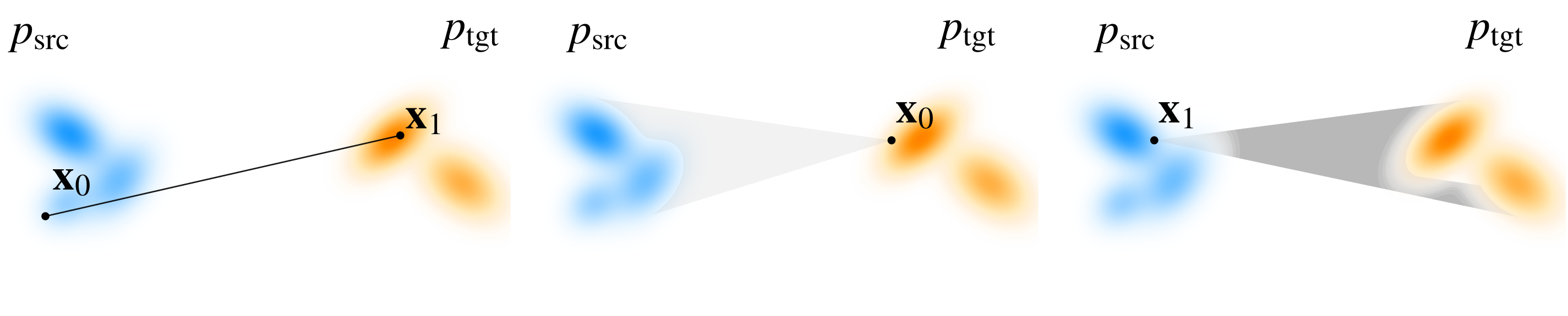
We aim to construct a conditional density path \(p_t(\cdot|{\mathbf{z}})\) first and then derive its corresponding conditional velocity field \({\mathbf{v}}_t(\cdot|{\mathbf{z}})\) (via Proposition: Closed-Form Velocity Field for Gaussian Density Path), under conditioning with respect to \(\pi({\mathbf{z}})\). Depending on how \({\mathbf{z}}\) is chosen, there are two natural scenarios: (i) two-sided conditioning with \({\mathbf{z}}=({\mathbf{x}}_0,{\mathbf{x}}_1)\), or (ii) one-sided conditioning with \({\mathbf{z}}={\mathbf{x}}_0\) or \({\mathbf{x}}_1\). In either case, the construction must match the boundary distributions: \[\begin{align*} p_{\mathrm{src}}({\mathbf{x}}_0) = \int p_0({\mathbf{x}}_0|{\mathbf{z}}) \pi({\mathbf{z}})\mathop{}\!\mathrm{d}{\mathbf{z}}, \quad p_{\mathrm{tgt}}({\mathbf{x}}_1) = \int p_1({\mathbf{x}}_1|{\mathbf{z}}) \pi({\mathbf{z}}) \mathop{}\!\mathrm{d}{\mathbf{z}}. \end{align*}\] Since verifying these constraints is straightforward once a concrete construction is specified, we do not emphasize the verification step here.
I. Two-Sided \({\mathbf{z}}= ({\mathbf{x}}_0, {\mathbf{x}}_1)\) — “Beam-Like” Path.
Choice of \(\pi({\mathbf{z}})\).
Consider general distributions \(p_{\mathrm{src}}\) and \(p_{\mathrm{tgt}}\) over \(\mathbb{R}^D\). Let \({\mathbf{z}}= ({\mathbf{x}}_0, {\mathbf{x}}_1)\) with \({\mathbf{x}}_0 \sim p_{\mathrm{src}}\) and \({\mathbf{x}}_1 \sim p_{\mathrm{tgt}}\) independently, i.e., \[\pi({\mathbf{z}}) = p_{\mathrm{src}}({\mathbf{x}}_0) p_{\mathrm{tgt}}({\mathbf{x}}_1).\]
Choice of Conditional Path \(p_t(\cdot|{\mathbf{z}})\).
Define the conditional path by linear interpolation with a fixed and small variance \(\sigma > 0\)8: \[p_t({\mathbf{x}}_t | {\mathbf{z}}= ({\mathbf{x}}_0, {\mathbf{x}}_1)) = \mathcal{N}({\mathbf{x}}_t; a_t{\mathbf{x}}_0 + b_t{\mathbf{x}}_1, \sigma^2 {\mathbf{I}}),\] where \(a_t\) and \(b_t\) are time-dependent functions satisfying \(a_0 = 1, b_0 = 0\) and \(a_1 = 0, b_1 = 1\). A choice suggested by (Lipman et al. 2022; Liu 2022) is \(a_t = 1-t\), \(b_t = t\). In the deterministic case \(\sigma = 0\), we obtain \[p_t({\mathbf{x}}_t |{\mathbf{z}}) = \delta \big({\mathbf{x}}_t - [a_t{\mathbf{x}}_0 + b_t{\mathbf{x}}_1]\big),\] which describes a deterministic interpolating path from \({\mathbf{x}}_0\) to \({\mathbf{x}}_1\).
Derived Conditional Velocity \({\mathbf{v}}_t(\cdot|{\mathbf{z}})\).
By Proposition: Closed-Form Velocity Field for Gaussian Density Path, the conditional velocity is \[{\mathbf{v}}_t({\mathbf{x}}| {\mathbf{z}}) = a'_t{\mathbf{x}}_0 + b'_t{\mathbf{x}}_1.\]
CFM Loss.
When \(\sigma=0\) so that \({\mathbf{x}}_t = a_t{\mathbf{x}}_0 + b_t{\mathbf{x}}_1\), the CFM loss reduces to \[\mathcal{L}_{\mathrm{CFM}} = \mathbb{E}_{t, {\mathbf{x}}_0\sim p_{\text{src}}, {\mathbf{x}}_1\sim p_{\text{tgt}}} \left\| {\mathbf{v}}_{\bm{\phi}}({\mathbf{x}}_t, t) - \left(a'_t{\mathbf{x}}_0 + b'_t{\mathbf{x}}_1\right) \right\|^2.\] From Equation and Equation, the optimal velocity field is \[{\mathbf{v}}^*({\mathbf{x}}_t, t) = \mathbb{E} \left[ {\mathbf{x}}_t'|{\mathbf{x}}_t \right] = \mathbb{E} \left[ a'_t{\mathbf{x}}_0 + b'_t{\mathbf{x}}_1|{\mathbf{x}}_t \right].\] Here, the expectation is taken over \(p(\mathbf{x}_0, \mathbf{x}_1|\mathbf{x}_t)\), the conditional distribution over source-target pairs \((\mathbf{x}_0, \mathbf{x}_1)\) that could have produced the observed interpolation \(\mathbf{x}_t = a_t\mathbf{x}_0 + b_t\mathbf{x}_1\) at time \(t\).
II. One-Sided \({\mathbf{z}}= {\mathbf{x}}_0\) or \({\mathbf{x}}_1\) — “Spotlight-Like” Path.
We illustrate the conditional probability–path–first construction in the one-sided setting, considering the standard generative setup with \(p_{\mathrm{src}}=\mathcal N(\bm 0,{\mathbf{I}})\) and \(p_{\mathrm{tgt}}=p_{\mathrm{data}}\). Crucially, this Gaussian source is not an additional assumption but a direct consequence of the conditional path defined below. A more general treatment of arbitrary endpoints will be given in Section 1.3.3.
Choice of \(\pi({\mathbf{z}})\).
We take \({\mathbf{z}}={\mathbf{x}}_1\) with \(\pi({\mathbf{z}})=p_{\mathrm{data}}({\mathbf{x}}_1)\) (the case \({\mathbf{z}}={\mathbf{x}}_0\sim p_{\mathrm{prior}}\) follows analogously).
Choice of Conditional Path \(p_t(\cdot|{\mathbf{z}})\).
For fixed \({\mathbf{x}}_1\sim p_{\mathrm{data}}\), define \[p_t({\mathbf{x}}_t|{\mathbf{z}}={\mathbf{x}}_1)=\mathcal N \big({\mathbf{x}}_t; b_t {\mathbf{x}}_1, a_t^2 {\mathbf{I}}\big),\] with \(a_0=1, b_0=0, a_1=0, b_1=1\) (usually interpreted as the limit). At the boundaries, \[p_0(\cdot|{\mathbf{z}}={\mathbf{x}}_1)=\mathcal N(\cdot; \bm 0,{\mathbf{I}}),\qquad p_1(\cdot|{\mathbf{z}}={\mathbf{x}}_1)=\delta(\cdot - {\mathbf{x}}_1).\] Marginalizing over \({\mathbf{x}}_1\) yields \(\{p_t\}_{t\in[0,1]}\) with \(p_0=\mathcal N(\bm 0,{\mathbf{I}})\) (independent of \(p_{\mathrm{data}}\)) and \(p_1=p_{\mathrm{data}}\).
Derived Conditional Velocity \({\mathbf{v}}_t(\cdot|{\mathbf{z}})\).
For \(t\in(0,1)\) with \(a_t>0\), applying Proposition: Closed-Form Velocity Field for Gaussian Density Path to the conditional Gaussian path gives \[\mathbf v_t({\mathbf{x}}|{\mathbf{x}}_1) = b_t' {\mathbf{x}}_1 + \frac{a_t'}{a_t} \big({\mathbf{x}}- b_t {\mathbf{x}}_1\big).\]
One-Sided CFM Objective.
With \(t\sim\mathcal U(0,1)\) (or any fixed sampling distribution) and \({\mathbf{x}}_1\sim p_{\mathrm{data}}\), the CFM loss becomes \[\begin{align} \label{eq:one-sided-cfm} \mathcal L_{\mathrm{CFM}} =\mathbb{E}_{t,{\mathbf{x}}_1} \mathbb{E}_{{\mathbf{x}}_t\sim p_t(\cdot|{\mathbf{x}}_1)} \Big\|\mathbf v_\phi({\mathbf{x}}_t,t)- \Big[b_t'{\mathbf{x}}_1+\tfrac{a_t'}{a_t}\big({\mathbf{x}}_t-b_t{\mathbf{x}}_1\big)\Big]\Big\|_2^2. \end{align}\] By MSE optimality, the unique minimizer is the marginal velocity field \[\mathbf v^*({\mathbf{x}},t) = \mathbb{E}\left[\mathbf v_t({\mathbf{x}}|{\mathbf{x}}_1) |dle| {\mathbf{x}}_t={\mathbf{x}}\right] = \mathbb{E}\left[a_t'{\mathbf{x}}_0+b_t'{\mathbf{x}}_1 |dle| {\mathbf{x}}_t={\mathbf{x}}\right].\]
Equivalence to Two-Sided Target.
For paired samples \(({\mathbf{x}}_0,{\mathbf{x}}_1)\) with \({\mathbf{x}}_t=a_t{\mathbf{x}}_0+b_t{\mathbf{x}}_1\), \[\mathbf v_t({\mathbf{x}}_t|{\mathbf{x}}_1) = b_t'{\mathbf{x}}_1 + \tfrac{a_t'}{a_t}\big({\mathbf{x}}_t-b_t{\mathbf{x}}_1\big) = a_t'{\mathbf{x}}_0 + b_t'{\mathbf{x}}_1.\] Thus the one-sided loss regresses to the conditional expectation of the two-sided target given \({\mathbf{x}}_t\): \[\mathbf v^*({\mathbf{x}},t)=\mathbb{E}\big[a_t'{\mathbf{x}}_0 + b_t'{\mathbf{x}}_1 | {\mathbf{x}}_t={\mathbf{x}}\big],\] so the one-sided and two-sided CFM objectives share the same minimizer.
Gaussian FM = Diffusion Model.
We use the FM convention where \(t=0\) denotes the source/prior and \(t=1\) denotes the target/data: \[p_{\mathrm{src}}=p_{\mathrm{prior}},\qquad p_{\mathrm{tgt}}=p_{\mathrm{data}}.\] By contrast, diffusion models typically index time from data to noise (i.e., \(t=0\) is data and \(t=1\) is prior). Here, we adopt the FM convention indexing in the main discussion. For comparison, however, the VE and VP entries in Table 1.2 are summarized in their usual diffusion-time indexing, where \(t=0\) corresponds to data and \(t=1\) to prior/noise. If further \(p_{\mathrm{src}}=\mathcal N(\bm 0,{\mathbf{I}})\), then for fixed condition \({\mathbf{x}}_1\sim p_{\mathrm{data}}\), the conditional path \(p_t(\cdot |{\mathbf{x}}_1)\) is naturally chosen to be Gaussian, while the target distribution \(p_{\mathrm{tgt}}\) itself need not be Gaussian. We refer to this Gaussian conditional-path setting as Gaussian FM. Diffusion probability paths form an important subclass of such Gaussian paths. A generic Gaussian schedule, however, need not correspond to a valid forward diffusion SDE; the schedule must additionally satisfy the SDE compatibility condition in Lemma in Chapter 4 (Forward Perturbation Kernel ⟺ Linear SDE).
Choosing \(a_t = 1-t\) and \(b_t = t\) (equivalently, \(\alpha_t = t\) and \(\sigma_t = 1-t\) under the relabeling \(a_t:=\sigma_t\), \(b_t:=\alpha_t\) in diffusion model) recovers the familiar FM/RF schedule (Lipman et al. 2022; Liu 2022).
| VE | VP | FM/RF | Trig. (Albergo et al. 2023) | |
|---|---|---|---|---|
| \(a_t\) (prior coeff.) | \(a_t\) | \(\sqrt{1-b_t^2}\) | \(1-t\) | \(\cos \bigl(\tfrac{\pi}{2}t\bigr)\) |
| \(b_t\) (data coeff.) | \(1\) | \(b_t\) | \(t\) | \(\sin \bigl(\tfrac{\pi}{2}t\bigr)\) |
| \(a_0\) | \(0\) | \(0\) | \(1\) | \(1\) |
| \(b_0\) | \(1\) | \(1\) | \(0\) | \(0\) |
| \(a_1\) | \(a_1\) | \(1\) | \(0\) | \(0\) |
| \(b_1\) | \(1\) | \(0\) | \(1\) | \(1\) |
| \(p_{\text{prior}}\) | \(p_{\mathrm{data}} * \mathcal{N}(\bm{0},a_1^2{\mathbf{I}}) \approx \mathcal{N}(\bm{0},a_1^2{\mathbf{I}})\) | \(\mathcal{N}(\bm{0},{\mathbf{I}})\) | \(\mathcal{N}(\bm{0},{\mathbf{I}})\) | \(\mathcal{N}(\bm{0},{\mathbf{I}})\) |
In the Gaussian FM setting, both the beam-like and spotlight-like conditional paths lead to training objectives that are similar to the standard diffusion losses. As we will elaborate in Chapter 6, Gaussian FM can in fact be equivalently interpreted as a diffusion model trained to predict the velocity, under the linear schedule \(a_t = 1-t\) and \(b_t = t\). This perspective highlights that flow matching and diffusion are not fundamentally different, but rather two equivalent formulations that can be transformed into one another. The Gaussian FM objective is particularly appealing in practice: its loss function (\(\mathbb{E}_{t,{\mathbf{x}}_t} \left[\left\lVert{\mathbf{v}}_{\bm{\phi}}({\mathbf{x}}_t, t) - ({\mathbf{x}}_1 - {\mathbf{x}}_0)\right\rVert_2^2\right]\)) is simple, and it has been shown to achieve competitive performance at scale (Esser et al. 2024).
Conditional Flow-First Construction of \({\mathbf{v}}_t(\cdot|{\mathbf{z}})\) and \(p_t(\cdot|{\mathbf{z}})\)
We treat the general case where the endpoints \(p_{\mathrm{src}}\) (at \(t=0\)) and \(p_{\mathrm{tgt}}\) (at \(t=1\)) are arbitrary. Our goal is to design, directly in trajectory space, a conditional flow that transports samples from \(p_{\mathrm{src}}\) to \(p_{\mathrm{tgt}}\) and yields a closed-form \({\mathbf{v}}_t({\mathbf{x}}_t|{\mathbf{z}})\) usable as a regression target.
Motivation.
Instead of first designing conditional density path, we may directly specify a conditional flow map \({\bm{\Psi}}_{0\to t}(\cdot;{\mathbf{z}})\) that moves samples along trajectories. This has two practical advantages: (i) it immediately yields a regression target for training via a time derivative along trajectories; (ii) on geometry-structured spaces (Riemannian manifolds, Lie groups, or constrained submanifolds), it is often natural to construct the conditional flow map \({\bm{\Psi}}_{0\to t}\) directly from the geometry (e.g., geodesics, exponential maps, or premetrics) (Lipman et al. 2024) which yields analytic, simulation-free target velocities for training.
Conditional Affine Flow (Link to Proposition: Closed-Form Velocity Field for Gaussian Density Path).
We fix a conditioning variable \({\mathbf{z}}\sim\pi\) (e.g., \({\mathbf{z}}={\mathbf{x}}_1\sim p_{\mathrm{tgt}}\) in one-sided “spotlight’’ training) and push forward \({\mathbf{x}}_0\sim p_{\mathrm{src}}\) through the time-varying conditional affine flow \[{\bm{\Psi}}_{0\to t}({\mathbf{x}}_0;{\mathbf{z}}) := \bm\mu_t({\mathbf{z}}) + {\mathbf{A}}_t({\mathbf{z}}) {\mathbf{x}}_0,\qquad t\in[0,1],\] where \(\bm\mu_t({\mathbf{z}})\in\mathbb{R}^D\) and \({\mathbf{A}}_t({\mathbf{z}})\in\mathbb{R}^{D\times D}\) is invertible for \(t\in(0,1)\). The boundary \({\mathbf{A}}_0({\mathbf{z}})={\mathbf{I}},\ \bm\mu_0({\mathbf{z}})=\mathbf 0\) recovers \(p_{\mathrm{src}}\) at \(t=0\). It is standard to interpret boundary when \(t\to1\) as a limit (the terminal map may concentrate mass on a lower-dimensional set or a point)9.
Induced Conditional Path \(p_t(\cdot|{\mathbf{z}})\).
The construction defines \[p_t(\cdot|{\mathbf{z}}) = \bigl({\bm{\Psi}}_{0\to t}( \cdot ;{\mathbf{z}})\bigr)_{\#} p_{\mathrm{src}}, \qquad p_t(\cdot) = \int p_t(\cdot|{\mathbf{z}})\pi({\mathbf{z}})\mathop{}\!\mathrm{d}{\mathbf{z}}.\] What ultimately matters in \(\mathcal{L}_{\mathrm{CFM}}\) is how to sample from it: first draw \({\mathbf{z}}\sim \pi\), then draw \({\mathbf{x}}_0 \sim p_{\mathrm{src}}\), and finally set \[{\mathbf{x}}_t = \bm\mu_t({\mathbf{z}}) + {\mathbf{A}}_t({\mathbf{z}}){\mathbf{x}}_0.\]
We remark that when \({\bm{\Psi}}_{0\to t}\) is affine in \({\mathbf{x}}_0\), then \(p_t( \cdot | {\mathbf{z}})\) is Gaussian if and only if \(p_{\mathrm{src}}\) is Gaussian. In particular, for arbitrary (non-Gaussian) \(p_{\mathrm{src}}\), an affine flow yields a generally non-Gaussian \(p_t(\cdot|{\mathbf{z}})\).
Derived Conditional Velocity \({\mathbf{v}}_t(\cdot|{\mathbf{z}})\).
The conditional velocity \({\mathbf{v}}_t(\cdot|{\mathbf{z}})\) is obtained by \(t\)-differentiating the conditional flow map \({\bm{\Psi}}_{0\to t}\). Following the derivation in Proposition: Closed-Form Velocity Field for Gaussian Density Path, consider the conditional ODE defined by the flow map \({\bm{\Psi}}_{0\to t}({\mathbf{y}};{\mathbf{z}})\) with initial condition \({\mathbf{y}}\), where the goal is to identify the corresponding conditional velocity field \({\mathbf{v}}_t(\cdot|{\mathbf{z}})\): \[\frac{\mathop{}\!\mathrm{d}}{\mathop{}\!\mathrm{d}t} {\bm{\Psi}}_{0\to t}({\mathbf{y}};{\mathbf{z}}) = {\mathbf{v}}_t \Big(\underbrace{{\bm{\Psi}}_{0\to t}({\mathbf{y}};{\mathbf{z}})}_{{\mathbf{x}}} \Big| {\mathbf{z}}\Big).\] Since \({\bm{\Psi}}_{0\to t}(\cdot;{\mathbf{z}})\) is invertible for \(t\in(0,1)\), we may express the initial point \({\mathbf{y}}\) corresponding to the current state \({\mathbf{x}}={\bm{\Psi}}_{0\to t}({\mathbf{y}};{\mathbf{z}})\) as \[{\mathbf{y}} = {\bm{\Psi}}_{0\to t}^{-1}({\mathbf{x}};{\mathbf{z}}) = {\bm{\Psi}}_{t\to0}({\mathbf{x}};{\mathbf{z}}).\] The corresponding Eulerian velocity field is therefore \[{\mathbf{v}}_t({\mathbf{x}}|{\mathbf{z}}) := \left. \frac{\partial}{\partial t} {\bm{\Psi}}_{0\to t}({\mathbf{y}};{\mathbf{z}}) \right|_{{\mathbf{y}}={\bm{\Psi}}_{0\to t}^{-1}({\mathbf{x}};{\mathbf{z}})}.\] That is, we first differentiate the forward flow map with respect to \(t\) while holding its initial point \({\mathbf{y}}\) fixed, and then substitute the initial point whose trajectory reaches \({\mathbf{x}}\) at time \(t\).
Since \({\mathbf{x}}_t=\bm\mu_t({\mathbf{z}})+{\mathbf{A}}_t({\mathbf{z}}){\mathbf{x}}_0\) and \({\mathbf{A}}_t({\mathbf{z}})\) is invertible on \((0,1)\), we have \({\mathbf{x}}_0={\mathbf{A}}_t({\mathbf{z}})^{-1}\bigl({\mathbf{x}}-\bm\mu_t({\mathbf{z}})\bigr)\), giving \[{\mathbf{v}}_t({\mathbf{x}}|{\mathbf{z}}) = \bm\mu_t'({\mathbf{z}}) + {\mathbf{A}}_t'({\mathbf{z}}) {\mathbf{A}}_t({\mathbf{z}})^{-1} \bigl({\mathbf{x}}-\bm\mu_t({\mathbf{z}})\bigr).\]
One-Sided Conditioning (\({\mathbf{z}}={\mathbf{x}}_1\)).
Choosing \(\bm\mu_t({\mathbf{z}})=b_t {\mathbf{z}}\) and \({\mathbf{A}}_t({\mathbf{z}})=a_t {\mathbf{I}}\) with \(a_0=1,a_1=0\) and \(b_0=0,b_1=1\) (with \(a_t>0\) for \(t\in(0,1)\)) yields \[{\mathbf{x}}_t = a_t {\mathbf{x}}_0 + b_t {\mathbf{x}}_1, \qquad {\mathbf{v}}_t({\mathbf{x}}|{\mathbf{x}}_1) = b_t' {\mathbf{x}}_1 + \frac{a_t'}{a_t} \bigl({\mathbf{x}}-b_t{\mathbf{x}}_1\bigr).\] On paired samples \(({\mathbf{x}}_0,{\mathbf{x}}_1)\) (with \({\mathbf{x}}_t=a_t{\mathbf{x}}_0+b_t{\mathbf{x}}_1\)), this simplifies to the usual CFM target: \[{\mathbf{v}}_t({\mathbf{x}}_t|{\mathbf{x}}_1)=a_t' {\mathbf{x}}_0 + b_t' {\mathbf{x}}_1.\]
Two-Sided Conditioning (\({\mathbf{z}}=({\mathbf{x}}_0,{\mathbf{x}}_1)\)).
The same template with \(\bm\mu_t({\mathbf{x}}_0,{\mathbf{x}}_1)=b_t {\mathbf{x}}_1\) and \({\mathbf{A}}_t({\mathbf{x}}_0,{\mathbf{x}}_1)=a_t {\mathbf{I}}\) makes the conditional path deterministic: \[{\mathbf{x}}_t=a_t {\mathbf{x}}_0+b_t {\mathbf{x}}_1, \qquad p_t(\cdot|{\mathbf{x}}_0,{\mathbf{x}}_1)=\delta\left(\cdot - (a_t{\mathbf{x}}_0+b_t{\mathbf{x}}_1)\right),\] and the conditional velocity is \[{\mathbf{v}}_t({\mathbf{x}}_t|{\mathbf{x}}_0,{\mathbf{x}}_1)=a_t' {\mathbf{x}}_0+b_t' {\mathbf{x}}_1,\] i.e., the standard two-sided CFM target.
Unconditional Gaussian Path as a Special Case.
If \(\bm{\mu}_t\) is independent of \({\mathbf{z}}\) (denoted \(\bm{\mu}(t)\)) and \({\mathbf{A}}_t = \tfrac{\sigma(t)}{\sigma(0)} {\mathbf{I}}\), then \[{\bm{\Psi}}_{0\to t}({\mathbf{x}}_0)=\bm\mu(t)+\sigma(t) \frac{{\mathbf{x}}_0-\bm\mu(0)}{\sigma(0)}, \quad {\mathbf{v}}_t({\mathbf{x}})=\bm\mu'(t)+\frac{\sigma'(t)}{\sigma(t)}\bigl({\mathbf{x}}-\bm\mu(t)\bigr),\] which recovers the Gaussian density path and the closed-form velocity in Proposition: Closed-Form Velocity Field for Gaussian Density Path.
Probability-Path-First vs. Flow-First Construction
The two constructions correspond to complementary Eulerian and Lagrangian descriptions of transport. The probability-path-first (Eulerian) view begins by specifying a conditional density path \(p_t(\cdot|{\mathbf{z}})\) and then selects a compatible velocity field through the continuity equation. Because a density path alone generally does not determine the velocity uniquely, additional transport structure may be needed to select one.
The flow-first (Lagrangian) view instead specifies a conditional flow map \({\bm{\Psi}}_{0\to t}(\cdot|{\mathbf{z}})\), which directly describes particle trajectories. The corresponding density path follows by pushforward, and when the map is invertible its Eulerian velocity is uniquely recovered as \[{\mathbf{v}}_t = \partial_t{\bm{\Psi}}_{0\to t} \circ {\bm{\Psi}}_{0\to t}^{-1}.\] Both constructions therefore describe the same kinds of transport objects from different starting points, but a prescribed density path need not select the same velocity as a separately prescribed flow map.
The following table summarizes these contrasts. The takeaway: path-first is natural when conditional paths admit closed-form velocities; flow-first is natural when you have strong structural priors on trajectories.
| Axis | Conditional Probability-Path-First | Conditional Flow-First |
|---|---|---|
| Given | Conditional density path \(p_t(\cdot|{\mathbf{z}})\). | Conditional flow map \({\bm{\Psi}}_{0\to t}(\cdot|{\mathbf{z}})\) (trajectories, for each fixed \({\mathbf{z}}\)). |
| Get Velocity | For each \({\mathbf{z}}\), find \({\mathbf{v}}_t(\cdot|{\mathbf{z}})\) s.t. \[\partial_t p_t(\cdot|{\mathbf{z}}) + \nabla \cdot \left( p_t(\cdot|{\mathbf{z}}){\mathbf{v}}_t(\cdot|{\mathbf{z}}) \right) = 0;\] Non-unique: if \(\nabla\!\cdot~\left(p_t \mathbf w_t\right)=0\) then \({\mathbf{v}}_t+\mathbf w_t\) yields the same \(p_t\). | Along paths (for each \({\mathbf{z}}\)): \[{\mathbf{v}}_t \left( {\bm{\Psi}}_{0\to t}(\cdot|{\mathbf{z}}) \mid {\mathbf{z}} \right) = \tfrac{\mathop{}\!\mathrm{d}}{\mathop{}\!\mathrm{d}t} {\bm{\Psi}}_{0\to t}(\cdot|{\mathbf{z}}).\] When \({\bm{\Psi}}_{0\to t}\) is invertible, one can solve \[{\mathbf{v}}_t({\mathbf{x}}|{\mathbf{z}}) = \left. \partial_t {\bm{\Psi}}_{0\to t}({\mathbf{y}}|{\mathbf{z}}) \right|_{{\mathbf{y}}={\bm{\Psi}}_{0\to t}^{-1}({\mathbf{x}}|{\mathbf{z}})}.\] |
| Closed Form of \({\mathbf{v}}_t(\cdot|{\mathbf{z}})\) |
Convenient when \(p_t(\cdot|{\mathbf{z}})\) is Gaussian / exponential-family; otherwise obtaining \({\mathbf{v}}_t(\cdot|{\mathbf{z}})\) is nontrivial. | Convenient when \({\bm{\Psi}}_{0\to t}(\cdot|{\mathbf{z}})\) has structure (affine/low-rank); avoids density evaluation. |
| Uniqueness of \({\mathbf{v}}_t(\cdot|{\mathbf{z}})\) |
For each \({\mathbf{z}}\), \({\mathbf{v}}_t(\cdot|{\mathbf{z}})\) is underdetermined unless a selection rule (e.g., potential flow / min. kinetic energy) is imposed. | Given \({\bm{\Psi}}_{0\to t}(\cdot|{\mathbf{z}})\), both \(p_t(\cdot|{\mathbf{z}})=({\bm{\Psi}}_{0\to t}(\cdot|{\mathbf{z}}))_\#p_0\) and the particle trajectories are determined. If the flow map is invertible, the corresponding Eulerian velocity field is uniquely determined; otherwise, a unique global Eulerian field need not exist. |
| Realizability | Must verify the constructed \({\mathbf{v}}_t(\cdot|{\mathbf{z}})\) solving the continuity equation on the intended support. | Holds by construction: \[p_t(\cdot|{\mathbf{z}}) = \left( {\bm{\Psi}}_{0\to t}(\cdot|{\mathbf{z}}) \right)_\# p_0(\cdot|{\mathbf{z}}).\] |
| Match \((p_{\mathrm{src}},p_{\mathrm{tgt}})\) |
Mix conditionals: \(p_{\mathrm{src}} = \int p_0(\cdot|{\mathbf{z}})\pi({\mathbf{z}})\mathop{}\!\mathrm{d}{\mathbf{z}},\) \(p_{\mathrm{tgt}} = \int p_1(\cdot|{\mathbf{z}})\pi({\mathbf{z}})\mathop{}\!\mathrm{d}{\mathbf{z}}.\) Under Gaussian–affine conditional paths with \({\mathbf{z}}\)-independent coefficients, \(p_{\mathrm{src}}\) can be forced to be Gaussian. For a general fixed endpoint \(p_{\mathrm{src}}\) (possibly non-Gaussian), the choice of \(p_t(\cdot|{\mathbf{z}})\) does not generally pin \(p_{\mathrm{src}}\). |
Set \({\bm{\Psi}}_{0\to 0}=\mathrm{Id}\) and choose boundary condition to hit any \(p_{\mathrm{tgt}}\). |
| Preferred Scenarios |
Diffusion-style constructions; analytic targets via conditional Gaussians \(p_t(\cdot|{\mathbf{z}})\). | Strong structural priors via maps \({\bm{\Psi}}_{0\to t}(\cdot|{\mathbf{z}})\); easy boundary control; accommodates singular/low-dimensional endpoints; natural for map-based regularization/transport costs. |
Conditional Straightness Does Not Imply Marginal-Flow Straightness
The canonical affine interpolation \[{\mathbf{x}}_t = (1-t){\mathbf{x}}_0+t{\mathbf{x}}_1\] has an appealing geometric property: conditioned on a particular endpoint pair \(({\mathbf{x}}_0,{\mathbf{x}}_1)\), the interpolation is a straight line with constant velocity \({\mathbf{x}}_1-{\mathbf{x}}_0\). This conditional notion of straightness is used extensively in Flow Matching and Rectified Flow.
It is important, however, to distinguish the straightness of these conditional interpolation paths from the straightness of the marginal ODE trajectories used at generation time. Under a coupling \(\pi({\mathbf{x}}_0,{\mathbf{x}}_1)\), the population-optimal marginal velocity is \[{\mathbf{v}}^\star({\mathbf{x}},t) = \mathbb{E} \left[ {\mathbf{x}}_1-{\mathbf{x}}_0 \,\middle|\, {\mathbf{x}}_t={\mathbf{x}} \right].\] The posterior over endpoint pairs generally changes with \(({\mathbf{x}},t)\). Consequently, the velocity encountered along a marginal ODE trajectory need not remain constant, even though every conditional interpolation used for training is a straight line.
Thus, choosing the canonical affine schedule alone does not imply
that the learned marginal ODE is exactly straight or that one Euler step
is exact. Rectified Flow addresses precisely this distinction: its
rectification or Reflow procedure changes the endpoint
coupling so that the induced causal flow can become progressively closer
to a straight flow (Liu et al.
2022).
The following example makes the distinction explicit.
Example: A Simple 1D Counterexample
Consider the one-dimensional setting with \[x_0 \sim \mathcal{N}(0, \sigma_0^2), \qquad x_1 \sim \mathcal{N}(0, \sigma_1^2),\] independent coupling, and the canonical affine interpolation \(x_t = (1-t)x_0 + tx_1\). Each conditional path \((1-t)x_0 + tx_1\) is a straight line in time. We now compute the induced marginal velocity field.
Since \((x_1 - x_0,\, x_t)\) is jointly Gaussian, the conditional expectation is linear in \(x\), so \[v^*(x,t) = \mathbb{E}[x_1 - x_0| x_t = x] = \frac{\operatorname{Cov}(x_1 - x_0,\, x_t)} {\operatorname{Var}(x_t)}\, x.\] A direct calculation gives \[\operatorname{Var}(x_t) = (1-t)^2\sigma_0^2 + t^2\sigma_1^2 =: V(t),\] and \[\operatorname{Cov}(x_1 - x_0,\, x_t) = t\sigma_1^2 - (1-t)\sigma_0^2 = \tfrac{1}{2} V'(t).\] Hence \[v^*(x,t) = \frac{V'(t)}{2V(t)}\, x.\]
The marginal ODE \[\frac{\mathop{}\!\mathrm{d}z_t}{\mathop{}\!\mathrm{d}t} = v^*(z_t, t)\] therefore has the exact solution \[z_t = z_0 \sqrt{\frac{V(t)}{V(0)}} = z_0 \sqrt{(1-t)^2 + \frac{\sigma_1^2}{\sigma_0^2}\, t^2}.\]
Now, a straight-line interpolation in time would require \(z_t\) to be affine in \(t\), namely \(z_t = (1-t)z_0 + t\,z_1\) for some endpoint \(z_1\). But \[\sqrt{(1-t)^2 + \frac{\sigma_1^2}{\sigma_0^2}\, t^2}\] is not affine in \(t\) for any positive \(\sigma_0, \sigma_1\). Thus the ODE trajectory is generally not a straight-line interpolation in time. We illustrate this phenomenon in Figure 1.10 with the example \(\sigma_0=2\) and \(\sigma_1=3\).
For example, when \(\sigma_0 = \sigma_1\), we have \(z_1 = z_0\), so a straight-line interpolation would simply be the constant path \(z_t = z_0\). In contrast, the actual ODE trajectory satisfies \[z_{1/2} = \frac{z_0}{\sqrt{2}} \neq z_0.\] Therefore, even though every conditional interpolation path is straight, the induced marginal ODE trajectory need not be.
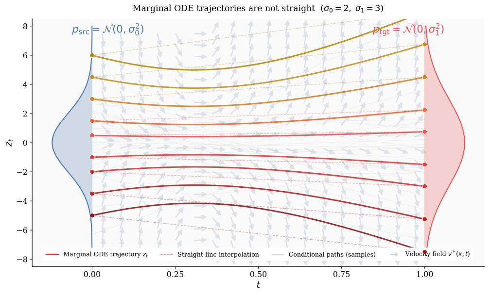
(Optional) Properties of the Canonical Affine Flow
Given two endpoint distributions \(p_0=p_{\mathrm{src}}\) and \(p_1=p_{\mathrm{tgt}}\), a natural and widely used choice for defining the conditional path in flow matching (FM) (Lipman et al. 2022) and rectified flow (RF) (Liu et al. 2022) is the linear interpolation \[a_t = 1 - t, \qquad b_t = t,\] which yields the interpolant \[\mathbf{x}_t = (1 - t)\mathbf{x}_0 + t \mathbf{x}_1, \qquad \mathbf{x}_0 \sim p_{\mathrm{src}},\ \mathbf{x}_1 \sim p_{\mathrm{tgt}}.\] Under this choice, the training objective simplifies to \[\mathbb{E}_{t \sim \mathcal{U}[0,1]} \mathbb{E}_{\mathbf{x}_0, \mathbf{x}_1} \left[ \bigl\|\mathbf{v}_{\bm{\phi}}(\mathbf{x}_t, t) - (\mathbf{x}_1 - \mathbf{x}_0)\bigr\|_2^2 \right].\]
This linear flow enjoys several appealing properties. In particular,
it admits an iterative refinement scheme, known as
Reflow, which progressively straightens the path
between distributions while preserving the marginals.
Rectifying Flows: From Noisy Guesses to Structured Pairings
Why Change the Coupling?
Under the independent coupling \[\pi({\mathbf{x}}_0,{\mathbf{x}}_1) = p_{\mathrm{src}}({\mathbf{x}}_0) p_{\mathrm{tgt}}({\mathbf{x}}_1),\] each conditional interpolation \((1-t){\mathbf{x}}_0+t{\mathbf{x}}_1\) is a straight line. As emphasized in Section 1.4, however, the corresponding marginal velocity averages directions from many unrelated endpoint pairs, so the induced marginal ODE trajectories need not be straight. Such curved marginal dynamics can be harder to integrate accurately with only a few numerical steps.
Rectification addresses this issue by changing the endpoint coupling. A learned ODE transports each source sample to a model-generated endpoint, producing a dependent coupling that is subsequently used to define a new conditional interpolation.
Rectify the Flow via Dependent Coupling.
Rather than relying on arbitrary pairings, we use a pre-trained diffusion model \({\mathbf{v}}_{{\bm{\phi}}^\times}(\cdot,t)\) as the drift in a PF-ODE to deterministically transport each source point. Starting from \({\mathbf{z}}(0)={\mathbf{z}}_0 \sim p_{\text{src}}\), we integrate \[\frac{\mathop{}\!\mathrm{d}{\mathbf{z}}(t)}{\mathop{}\!\mathrm{d}t} = {\mathbf{v}}_{{\bm{\phi}}^\times}({\mathbf{z}}(t),t), \qquad t \in [0,1],\] to obtain \(\hat{\mathbf{z}}_1 := {\mathbf{z}}(1)\) positioned near the data space learned from the pre-trained model. The resulting pair \(({\mathbf{z}}_0,\hat{\mathbf{z}}_1)\) forms a dependent coupling: it follows a structured, model-guided path rather than an arbitrary interpolation. This idea extends naturally to affine reference paths of the form \({\mathbf{x}}_t = a_t {\mathbf{x}}_0 + b_t {\mathbf{x}}_1\), where \({\mathbf{x}}_0 \sim p_{\text{src}}\) and \({\mathbf{x}}_1 \sim p_{\text{tgt}}\).
Algorithm: Rectify Operation
Input: Reference path \(\{{\mathbf{x}}_t\}_{t\in[0,1]}\) (e.g. \({\mathbf{x}}_t=a_t{\mathbf{x}}_0+b_t{\mathbf{x}}_1\))
Pre-Train Diffusion. Fit \({\mathbf{v}}_{{\bm{\phi}}^\times}\) on the chosen path by minimizing \[{\bm{\phi}}^\times \in \arg\min_{{\bm{\phi}}} \mathbb{E}_{t,{\mathbf{x}}_0,{\mathbf{x}}_1} \left[\Big\|{\mathbf{v}}_{{\bm{\phi}}}({\mathbf{x}}_t,t)-\frac{\mathop{}\!\mathrm{d}{\mathbf{x}}_t}{\mathop{}\!\mathrm{d}t}\Big\|_2^2\right].\]
Rectify. Sample \({\mathbf{z}}_0 \sim p_{\text{src}}\) and integrate \[\frac{\mathop{}\!\mathrm{d}{\mathbf{z}}(t)}{\mathop{}\!\mathrm{d}t}={\mathbf{v}}_{{\bm{\phi}}^\times}({\mathbf{z}}(t),t),\qquad {\mathbf{z}}(0)={\mathbf{z}}_0,\quad t\in[0,1],\] to obtain \(\hat{\mathbf{z}}_1={\mathbf{z}}(1)\) and the trajectory \(\{{\mathbf{z}}(t)\}_{t\in[0,1]}\). Output: Dependent (coherent) pair \(({\mathbf{z}}_0,\hat{\mathbf{z}}_1)\) or the full trajectory.
Why It Works: Marginal-Preserving Structure.
Let \({\bm{\Phi}}_{0\to t}\) denote
the flow map generated by the above ODE defined by the pre-trained
diffusion \({\mathbf{v}}_{{\bm{\phi}}^\times}\); then
\({\mathbf{z}}(t)={\bm{\Phi}}_{0\to
t}({\mathbf{z}}_0)\) and \(\hat{\mathbf{z}}_1={\bm{\Phi}}_{0\to
1}({\mathbf{z}}_0)\). The Rectify procedure pairs
each source point with its flow endpoint, giving the deterministic joint
\[\pi_{\text{Rectify}}({\mathbf{z}}_0,{\mathbf{z}}_1)
= p_{\text{src}}({\mathbf{z}}_0) \delta
\big({\mathbf{z}}_1-{\bm{\Phi}}_{0\to 1}({\mathbf{z}}_0)\big).\]
We have two immediate consequences:
Source Marginal is Preserved: \(\displaystyle \int \pi_{\text{Rectify}}({\mathbf{z}}_0,{\mathbf{z}}_1) \mathop{}\!\mathrm{d}{\mathbf{z}}_1 = p_{\text{src}}({\mathbf{z}}_0)\).
Pushforward Along the Flow: \(\displaystyle ({\bm{\Phi}}_{0\to t})_{\#}p_{\text{src}}=\mathrm{Law}({\mathbf{z}}(t))\), i.e., the time–\(t\) distribution is the pushforward of \(p_{\text{src}}\) by \({\bm{\Phi}}_{0\to t}\).
If \({\mathbf{v}}_{{\bm{\phi}}^\times}\) matches the oracle drift of a given reference path \({\mathbf{x}}_t\), then all intermediate marginals coincide: \[\mathrm{Law}({\mathbf{z}}(t))=\mathrm{Law}({\mathbf{x}}_t),\quad \text{for all }t\in[0,1], \quad\text{and}\quad ({\bm{\Phi}}_{0\to 1})_{\#}p_{\mathrm{src}}=p_{\mathrm{tgt}}.\]
Summary.
Rectification replaces the independent endpoint coupling with a
coupling induced by the learned flow. Under repeated
Reflow, this can produce marginal transport that is
progressively easier to integrate with few numerical steps.
For the canonical path, repeatedly applying Rectify
(“Reflow”) further straightens trajectories
without increasing transport cost, making training still easier.
Reflow: Iteratively
Straightening Flows
Why Reflow?
Independent pairings often induce irregular and meandering ODE trajectories between \(p_{\text{src}}\) and \(p_{\text{tgt}}\), which increase discretization error and variance during simulation. This raises a natural question:
Can we learn couplings that induce transport paths that are closer to straight lines between the two distributions, while still preserving the correct marginals?
This motivates Reflow: repeatedly apply
Rectify to update the coupling so that successive flows
become easier to integrate.
Core Idea:
Recursive Straightening via Rectify.
Start from the canonical interpolation on the product coupling \(\pi^{(0)}:=p_{\text{src}}({\mathbf{x}}_0)p_{\text{tgt}}({\mathbf{x}}_1)\),
\[{\mathbf{x}}_t=(1-t){\mathbf{x}}_0+t{\mathbf{x}}_1.\]
Applying Rectify replaces the independent pairing with a
dependent one \(({\mathbf{z}}_0,\hat{\mathbf{z}}_1)\)
induced by the learned ODE. Repeating this procedure, known as
Reflow, tends to produce straighter trajectories
that are easier to integrate accurately with a small number of numerical
steps. The precise straightening guarantee is discussed later in
Section 1.4.3.
The Reflow Procedure.
Each iteration performs two steps:
Re-Fit Flow: Train a new velocity field from samples of the current coupling: \[\begin{align} \bm{\phi}_{k+1} &= \arg\min_{\bm{\phi}} \mathcal{L}\left(\bm{\phi}\Big\vert \pi^{(k)}\right), \quad \text{where} \notag \\ \mathcal{L}\left(\bm{\phi}\Big\vert \pi^{(k)}\right) &:= \mathbb{E}_{t, ({\mathbf{z}}_0^{(k)}, \hat{\mathbf{z}}_1^{(k)})\sim \pi^{(k)}} \left[\left\|{\mathbf{v}}_{\bm{\phi}}({\mathbf{z}}_t, t) - (\hat{\mathbf{z}}_1^{(k)} - {\mathbf{z}}_0^{(k)})\right\|^2\right] \label{eq:reflow-loss} \end{align}\] with \({\mathbf{z}}_t = (1-t){\mathbf{z}}_0^{(k)} + t\hat{\mathbf{z}}_1^{(k)}\).
Generate New Coupling: Solve the learned ODE starting from new source samples \({\mathbf{z}}_0^{(k+1)} \sim p_{\text{src}}\): \[\hat{\mathbf{z}}_1^{(k+1)} \gets {\mathbf{z}}_0^{(k+1)} + \int_0^1 {\mathbf{v}}_{\bm{\phi}_{k+1}}({\mathbf{z}}(t), t) \mathrm{d}t,\] and define the updated coupling: \[\pi^{(k+1)}({\mathbf{z}}_0, {\mathbf{z}}_1) := p_{\text{src}}({\mathbf{z}}_0) \delta\left({\mathbf{z}}_1 - \hat{\mathbf{z}}_1^{(k+1)}\right).\]
In other words, Reflow can be viewed as repeatedly
applying the Rectify operator, producing a sequence of
progressively refined couplings: \[\begin{align}
\label{eq:rectify-op}
\pi^{(k+1)} = \texttt{Rectify} \left(\pi^{(k)}\right)
\end{align}\] so that both the flow and the coupling evolve
together, yielding progressively more stable transport paths.
Properties of Reflow
Two key theoretical properties drive the usefulness of
Reflow: it reduces transport cost and it straightens the
trajectories.
I.
Reflow Never Increases Transport Cost.
Let \(c({\mathbf{y}})\) be a convex
cost function (e.g., \(\|{\mathbf{y}}\|_2^p\) with \(p \geq 1\)). Each Rectify step
forms a new coupling \(({\mathbf{z}}_0,
\hat{\mathbf{z}}_1)\) whose cost is no worse than the
original:
Proposition: Rectify May Reduce Transport
Costs
Assuming an ideal velocity field \({\mathbf{v}}^* = {\mathbf{v}}_{\bm{\phi}^\times}\), we have: \[\mathbb{E}\left[c\left(\hat{\mathbf{z}}_1 - {\mathbf{z}}_0\right)\right] \leq \mathbb{E}\left[c\left({\mathbf{x}}_1 - {\mathbf{x}}_0\right)\right].\]
Proof for Proposition. Follows from Jensen’s inequality. See Liu et al. (2022) for a full derivation. ■
Applying this result recursively shows that the Reflow
process does not increase the transport cost.
II. Reflow
Straightens the Path.
Recursive application of Reflow promotes increasingly
straight trajectories, although the straightness measure is not
guaranteed to improve monotonically at every iteration. To measure this,
define the straightness functional of a path \(\mathbf{Y} =
\{{\mathbf{y}}_t\}_{t\in[0,1]}\) as \[\mathcal{S}(\mathbf{Y}) := \int_0^1
\mathbb{E}\left[\left\|{\mathbf{y}}_1 - {\mathbf{y}}_0 -
\frac{\mathrm{d}{\mathbf{y}}_t}{\mathrm{d}t} \right\|_2^2
\right] \mathrm{d}t.\] If \(\mathcal{S}(\mathbf{Y}) = 0\), then \(\mathbf{Y}\) is exactly a straight
line.
Proposition: Reflow Straightens the Stochastic
Path
For rectified paths \({\mathbf{Z}}^{(k)}\), we have: \[\min_{k \in \{0,\dots,K\}} \mathcal{S}({\mathbf{Z}}^{(k)}) \leq \frac{\mathbb{E}\left[\|{\mathbf{x}}_1 - {\mathbf{x}}_0\|^2\right]}{K}.\]
Proof for Proposition. See Theorem 3.7 of Liu et al. (2022). ■
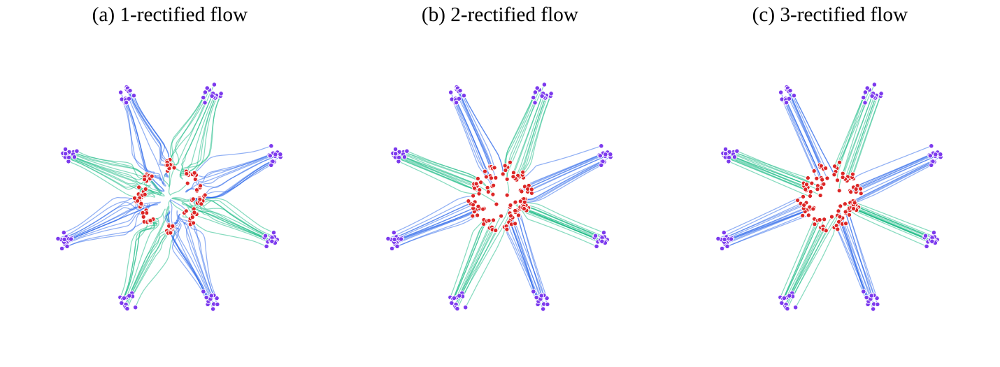
Reflow. Paths
become progressively straighter with Rectify procedure.
The FM or RF formulation with linear interpolation kernels, together
with the Reflow procedure, provides a simpler training
objective and a practical method for refining stochastic couplings. For
theoretical details, we refer readers to (Liu et
al. 2022; Liu 2022).
III. Connection to Optimal Transport.
Lastly, we note that straight-line couplings are not necessarily optimal in the sense of optimal transport (OT). This involves some terminology that will be introduced in Section (Taxonomy of the Problem Setups) in Chapter 7; we therefore refer readers who are not familiar with OT to that section.
A hallmark of quadratic-cost optimal transport is that particles travel along straight lines: a particle at \({\mathbf{x}}_0\) moves to \({\mathbf{T}}({\mathbf{x}}_0)\) via \({\mathbf{x}}_t = (1 - t){\mathbf{x}}_0 + t {\mathbf{T}}({\mathbf{x}}_0)\), where \({\mathbf{T}}\) is the optimal transport map. However, not every map \({\mathbf{S}}\) generating such straight-line paths, i.e., \({\mathbf{x}}_t = (1 - t){\mathbf{x}}_0 + t {\mathbf{S}}({\mathbf{x}}_0)\), is optimal. The map \({\mathbf{S}}\) yields the optimal flow only if it minimizes the Monge cost \(\mathbb{E}[\|{\mathbf{x}}_0 - {\mathbf{S}}({\mathbf{x}}_0)\|^2]\). Thus, while straight-line paths are necessary, they are not sufficient; optimality also depends on the correct endpoint map \({\mathbf{T}}\).
Example: Straight Couplings Need Not Be Optimal
Let \(p_{\text{src}} = p_{\text{tgt}} = \mathcal{N}(\bm{0}, {\mathbf{I}})\). For the cost \(c({\mathbf{x}}, {\mathbf{y}}) = \|{\mathbf{x}}- {\mathbf{y}}\|^p\) with \(p > 0\), the \(c\)-optimal coupling is the identity coupling \(\pi^{*}\), where \(\pi^{*}\) is the law of \(({\mathbf{x}}, {\mathbf{x}})\) with \({\mathbf{x}}\sim p_{\text{src}}\).
Now consider the coupling \(\pi_{{\mathbf{A}}}\) defined as the law of \(({\mathbf{x}}, {\mathbf{A}}{\mathbf{x}})\), where \({\mathbf{x}}\sim p_{\text{src}}\) and \({\mathbf{A}}\) is a rotation matrix satisfying \({\mathbf{A}}^\top {\mathbf{A}}= {\mathbf{I}}\), \(\det({\mathbf{A}}) = 1\), \({\mathbf{A}}\neq {\mathbf{I}}\), and \(-1\) is not an eigenvalue. Then \(\pi_{{\mathbf{A}}}\) is a valid coupling of \(p_{\text{src}}\) and \(p_{\text{tgt}}\), and corresponds to straight-line paths between \({\mathbf{x}}\) and \({\mathbf{A}}{\mathbf{x}}\), but it is not \(c\)-optimal for any twice-differentiable strictly convex cost \(c\) with invertible Hessian. The suboptimality arises from the rotational transformation. As discussed in Equation in Chapter 7, even removing the rotation may not lead to an optimal coupling.
We will continue exploring the connection to OT in Section (Can Canonical Linear Flow and Reflow Leads to an OT Map?) in Chapter 7.
Closing Remarks
This chapter has illuminated the third and final foundational perspective on diffusion models, one rooted in the principles of deterministic flows. Our exploration began with Normalizing Flows (NFs), which leverage the change-of-variables formula to learn an exact, invertible mapping between a simple prior and the data distribution. We then saw this concept evolve into a continuous-time process with Neural ODEs, where a learned velocity field governs the transformation. However, this approach comes with the significant drawback of requiring costly ODE simulations within the training loop.
The modern framework of Flow Matching (FM) was presented as an elegant and efficient solution to this challenge. By pre-defining a probability path \(\{p_{t}\}_t\) and a corresponding velocity field that satisfies the continuity equation, FM establishes a clear target for the ODE flow. Crucially, just as we saw in the variational and score-based views, FM employs a powerful conditioning trick. This transforms the intractable problem of matching the marginal velocity field into a simple and tractable regression against a known conditional velocity, making training entirely simulation-free. This perspective recasts diffusion models themselves as a special case of learning a deterministic flow to transport a Gaussian prior to the data distribution.
With the introduction of the flow-based view, our survey of the three conceptual pillars of diffusion modeling is now complete. Throughout this journey, a remarkable pattern has emerged: each framework, despite its unique origins in VAEs, EBMs, or NFs, has converged on a continuous-time generative process and has relied on a conditioning strategy to enable tractable learning.
In the next chapter, we will finally synthesize these parallel threads into a single, unified framework. We will:
Formally demonstrate that the variational, score-based, and flow-based perspectives are not merely analogous but are mathematically equivalent at a fundamental level.
Show how the Fokker-Planck equation serves as the universal law governing density evolution across all three views, revealing that they are simply different lenses for describing the same core generative principle.
This unified lens will provide a complete and systematic understanding of the modern diffusion paradigm.
If the map is further constrained to be the gradient of a convex potential, \({\mathbf{f}}_{\bm{\phi}}= \nabla \psi_{\bm{\phi}}\) with \(\psi_{\bm{\phi}}\) convex, then Equation \(\eqref{eq:nf-change-of-var-log}\) reduces to the Monge–Ampère relation in Equation in Chapter 7. This PDE characterizes the optimal transformation of one distribution into another under the quadratic cost. See Chapter 7 and (Huang et al. 2021) for further details.↩︎
We adopt a flipped time convention, with \(t = 0\) denoting the prior (source) and \(t = 1\) the data (target) distribution. The prior is interchangeably written as \(p_{\bm{\phi}}({\mathbf{x}}(0), 0)\), \(p_{\text{prior}}({\mathbf{x}}(0), 0)\), or simply \(p_{\text{prior}}({\mathbf{z}})\).↩︎
Several related approaches share the core idea of transporting between endpoint distributions using a continuous-time flow, although their formulations differ slightly. These include Flow Matching (FM) (Lipman et al. 2022; Neklyudov et al. 2023), Rectified Flow (RF) (Liu 2022; Heitz et al. 2023), and Stochastic Interpolants (Albergo et al. 2023; Albergo and Vanden-Eijnden 2023; Ma et al. 2024). Here, we use FM as a unifying terminology.↩︎
To align with the standard notation in FM literature, we reverse the time axis compared to earlier sections: \(t=0\) corresponds to the source distribution and \(t=1\) to the target.↩︎
The key distinction is that a probability path specifies the evolution of the distribution, but generally not the particle-level transport that realizes it. A particular velocity becomes determined only after additional transport structure is specified. For example, a sufficiently regular and invertible flow map \({\bm{\Psi}}_{0\to t}\) determines its Eulerian velocity through \(\mathbf{v}_t=\partial_t{\bm{\Psi}}_{0\to t}\circ{\bm{\Psi}}_{0\to t}^{-1}\). Likewise, once a forward diffusion SDE is specified, its associated PF-ODE selects the particular velocity \(\mathbf{v}_t(\mathbf{x}) = f(t)\mathbf{x} -\tfrac12g^2(t)\nabla_{\mathbf{x}}\log p_t(\mathbf{x})\). Thus, both cases add particle-level transport structure beyond the marginal path \(\{p_t\}\) itself.↩︎
The deterministic analogue of the Fokker–Planck equation, without the diffusion term.↩︎
In (Lipman et al. 2022), the authors consider \(\bm{\Psi}_{0\to t}({\mathbf{x}}) = \bm{\mu}(t) + \sigma(t){\mathbf{x}}\), which requires constraints on \(\bm{\mu}(t)\) and \(\sigma(t)\) to ensure boundary conditions. We adopt an equivalent normalized formulation that avoids such constraints.↩︎
One may instead add a fixed conditional variance \(\sigma^2{\mathbf{I}}\). The conditional velocity remains \(a_t'{\mathbf{x}}_0+b_t'{\mathbf{x}}_1\) because the variance is constant in time, but the endpoint marginals then become Gaussian smoothings of \(p_{\mathrm{src}}\) and \(p_{\mathrm{tgt}}\), approaching the desired endpoints as \(\sigma\to0\).↩︎
Allowing \({\mathbf{A}}_1({\mathbf{z}})\) to be singular (e.g., \(\mathbf 0\)) is compatible with invertibility on \((0,1)\) and causes the path to contract onto the prescribed endpoint at \(t=1\).↩︎