Chapter 8: Guidance and Controllable Generation

Diffusion models are powerful generative frameworks. In the unconditional setting, the goal is to learn \(p_{\text{data}}({\mathbf{x}})\) and generate samples without external input.

Many applications, however, require conditional generation, where outputs satisfy user-specified criteria. This can be achieved by steering an unconditional model or directly learning the conditional distribution \(p_0({\mathbf{x}}| {\mathbf{c}})\), with condition \({\mathbf{c}}\) (e.g., label, text description, or sketch) guiding the process.

This chapter builds on a principled view of the conditional score, which decomposes into an unconditional direction and a guidance direction that nudges samples toward the condition while preserving realism. We explain why guidance is essential, show how the conditional score serves as a unifying interface for control, and survey ways to approximate or replace the guidance term. We then distinguish control (meeting the condition) from alignment (meeting human preference under the condition), and describe how preferences can be incorporated into the same framework. Finally, we discuss direct optimization of preference without additional reward models (i.e., a learned scorer that assigns higher values to outputs better aligned with human preference).

Prologue

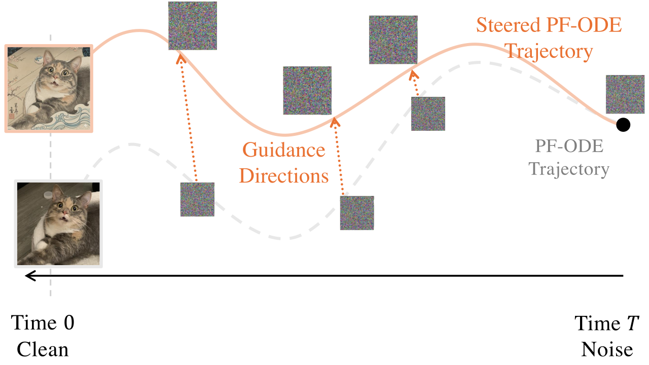
The generation process of diffusion models proceeds in a coarse-to-fine manner, providing a flexible framework for controllable generation. At each step, a small amount of noise is removed and the sample becomes clearer, gradually revealing more structure and detail. This property enables control over the generation process: by adding a guidance term to the learned, time-dependent velocity field, we can steer the generative trajectory to reflect user intent.

A principled foundation for guidance-based sampling in diffusion models is the Bayesian decomposition of the conditional score. For each noise level \(t\),

This identity shows that the exact conditional reverse dynamics are obtained by adding the guidance term \(\nabla_{{\mathbf{x}}_t}\log p_t({\mathbf{c}}|{\mathbf{x}}_t)\) on top of the unconditional score. We will see later on that classifier guidance (Dhariwal and Nichol 2021) estimates this term directly, classifier-free guidance (Ho and Salimans 2021) estimates it implicitly as the difference between jointly learned conditional and unconditional scores, and more general training-free methods may instead use a task-specific surrogate guidance direction.

With the exact conditional score, the PF-ODE becomes \[\begin{align} \label{eq:condition_prob_ode} \begin{aligned} \frac{\mathop{}\!\mathrm{d}\mathbf{x}(t)}{\mathop{}\!\mathrm{d}t} &= f(t)\mathbf{x}(t) - \frac{1}{2} g^2(t) \underbrace{\nabla_{{\mathbf{x}}_t} \log p_t({\mathbf{x}}(t) |{\mathbf{c}})}_{\text{conditional score}} \\ &= f(t)\mathbf{x}(t) - \frac{1}{2} g^2(t) \Big[ \nabla_{{\mathbf{x}}_t} \log p_t({\mathbf{x}}(t)) + \nabla_{{\mathbf{x}}_t} \log p_t({\mathbf{c}}|{\mathbf{x}}(t)) \Big]. \end{aligned} \end{align}\] With exact scores and exact integration, these dynamics recover \(p_0({\mathbf{x}}_0|{\mathbf{c}})\) when initialized from the corresponding terminal marginal \(p_T({\mathbf{x}}_T|{\mathbf{c}})\). In standard diffusion constructions, the terminal noising is chosen so that \(p_T({\mathbf{x}}_T|{\mathbf{c}})\) is approximately matched by the usual condition-independent prior.

We formulate the discussion below in score prediction for clarity. Since the standard \({\mathbf{x}}\)-, \({\bm{\epsilon}}\)-, score-, and \({\mathbf{v}}\)-prediction parameterizations are related by time-dependent linear transformations wherever these conversions are well-defined, the same guidance correction can be expressed in the other parameterizations using the relationships in Equation in Chapter 6.

Instantiations of the Guidance Direction.

1. Classifier Guidance (CG). In Section 1.2, classifier guidance (CG) trains a time-conditional classifier \(p_{{\bm{\psi}}}({\mathbf{c}}| {\mathbf{x}}_t, t)\) on noised data \({\mathbf{x}}_t\) (obtained by corrupting clean labeled samples at level \(t\)). At sampling time, its input gradient provides the guidance term: \[\nabla_{{\mathbf{x}}_t}\log p_{{\bm{\psi}}}({\mathbf{c}}| {\mathbf{x}}_t, t) \approx \nabla_{{\mathbf{x}}_t}\log p_t({\mathbf{c}}| {\mathbf{x}}_t),\] which is then added to the unconditional score (Dhariwal and Nichol 2021).

2. Classifier-Free Guidance (CFG). In Section 1.3, CFG directly trains a single conditional model \[{\mathbf{s}}_{{\bm{\phi}}}({\mathbf{x}}_t,t,{\mathbf{c}}) \approx \nabla_{{\mathbf{x}}_t}\log p_t({\mathbf{x}}_t|{\mathbf{c}}),\] where the unconditional model is learned jointly by randomly replacing the condition with a special null token for a fraction of the training steps.

3. Training-Free (Surrogate) Guidance. Under the standard forward noising construction, we first draw \(({\mathbf{x}}_0,{\mathbf{c}})\sim p_{\mathrm{data}}\) and then sample \({\mathbf{x}}_t\sim p_t(\cdot|{\mathbf{x}}_0)\), where the forward kernel does not depend additionally on \({\mathbf{c}}\). Thus \({\mathbf{c}}\perp{\mathbf{x}}_t\mid{\mathbf{x}}_0\)¹. Consequently, \[p_t({\mathbf{c}}|{\mathbf{x}}_t) = \int p({\mathbf{c}}|{\mathbf{x}}_0)\, p({\mathbf{x}}_0|{\mathbf{x}}_t)\, \mathrm d{\mathbf{x}}_0.\] This posterior average is generally intractable, motivating training-free methods that instead construct a task-specific surrogate guidance direction.

   In Section 1.4.1, training-free (loss-based) guidance avoids evaluating the conditional likelihood \(p_t({\mathbf{c}}|{\mathbf{x}}_t)\) directly. Instead, it starts from an off-the-shelf loss \(\ell({\mathbf{x}}_t,{\mathbf{c}};t)\) that measures how well the current sample satisfies the desired condition, with smaller loss indicating better agreement. From this loss, we define the positive guidance potential \[{\mathbf{h}}_t({\mathbf{x}}_t;{\mathbf{c}}) := \exp\big(-\tau\,\ell({\mathbf{x}}_t,{\mathbf{c}};t)\big), \qquad \tau>0.\] Thus, lower-loss samples receive larger potential values. We denote the corresponding guidance direction by \[\mathcal{G}_t({\mathbf{x}}_t,{\mathbf{c}}) := \nabla_{{\mathbf{x}}_t}\log {\mathbf{h}}_t({\mathbf{x}}_t;{\mathbf{c}}) = -\tau\nabla_{{\mathbf{x}}_t}\ell({\mathbf{x}}_t,{\mathbf{c}};t).\]

   Classifier guidance fits naturally into the same picture. At the population level, its guidance potential is \[{\mathbf{h}}_t({\mathbf{x}}_t;{\mathbf{c}}) = p_t({\mathbf{c}}|{\mathbf{x}}_t),\] which is approximated in practice by the learned classifier \(p_{{\bm{\psi}}^\times}({\mathbf{c}}|{\mathbf{x}}_t,t)\). Equivalently, the learned classifier corresponds to the loss \[\ell({\mathbf{x}}_t,{\mathbf{c}};t) = -\log p_{{\bm{\psi}}^\times}({\mathbf{c}}|{\mathbf{x}}_t,t), \qquad \tau=1.\]

At the population level, the three constructions above share the same additive guidance template. Given a positive potential \({\mathbf{h}}_t({\mathbf{x}}_t;{\mathbf{c}})\) and guidance strength \(w_t\geq0\), define the guided score field \[\begin{align} {\mathbf{s}}^{\mathrm{guide}}({\mathbf{x}}_t,t,{\mathbf{c}};w_t) := \nabla_{{\mathbf{x}}_t}\log p_t({\mathbf{x}}_t) + w_t\mathcal{G}_t({\mathbf{x}}_t,{\mathbf{c}}). \label{eq:generic-guided-score} \end{align}\] For loss-based guidance, \(\mathcal{G}_t({\mathbf{x}}_t,{\mathbf{c}}) =-\tau\nabla_{{\mathbf{x}}_t}\ell({\mathbf{x}}_t,{\mathbf{c}};t)\). For exact classifier guidance, \(\mathcal{G}_t({\mathbf{x}}_t,{\mathbf{c}}) =\nabla_{{\mathbf{x}}_t}\log p_t({\mathbf{c}}|{\mathbf{x}}_t)\); classifier-free guidance expresses the same population guidance direction through the difference between conditional and unconditional scores.

At each fixed time \(t\), Equation \(\eqref{eq:generic-guided-score}\) is, whenever normalizable, the score of the tilted density \[\widetilde p_t^{\mathrm{tilt}}({\mathbf{x}}_t|{\mathbf{c}}) \propto p_t({\mathbf{x}}_t){\mathbf{h}}_t({\mathbf{x}}_t;{\mathbf{c}})^{w_t}.\] This gives a useful energy interpretation: the base density favors samples supported by the diffusion model, while the potential reweights them toward the desired condition.

In practice, the corresponding learned or surrogate version of Equation \(\eqref{eq:generic-guided-score}\) is inserted into the reverse-time dynamics. Importantly, the tilted density above is only a fixed-time interpretation: the family \(\{\widetilde p_t^{\mathrm{tilt}}(\cdot|{\mathbf{c}})\}_t\) need not coincide with the marginals generated by the guided sampler. Consequently, for a generic loss or guidance schedule, integrating the guided PF-ODE from \(T\) to \(0\) does not in general produce samples distributed according to \(\widetilde p_0^{\mathrm{tilt}}(\cdot|{\mathbf{c}})\). The additional cross-time consistency required for this interpretation to hold is discussed in Section 1.4.2.

The effect of guidance on the sampling trajectory is illustrated in Figure 1.1. The same principle can also be applied on top of an already conditional model, allowing additional control signals to modify its sampling dynamics.

From Control to Better Alignment with Direct Preference Optimization.

Strong control can be on-condition but off-preference: a sample may satisfy the conditioning signal (e.g., the prompt) yet deviate from what humans actually prefer. We formalize this by tilting the conditional target at \(t=0\) by a preference rating: \[\widetilde p_0^{\mathrm{tilt}}({\mathbf{x}}_0|{\mathbf{c}}) \propto p_0({\mathbf{x}}_0|{\mathbf{c}}) \exp\bigl( \lambda_{\mathrm{pref}} r({\mathbf{x}}_0,{\mathbf{c}}) \bigr), \qquad \lambda_{\mathrm{pref}}>0,\] where \(r({\mathbf{x}}_0,{\mathbf{c}})\) is a scalar alignment rating for a clean sample \({\mathbf{x}}_0\) and condition \({\mathbf{c}}\), with larger values indicating stronger preference, and \(\lambda_{\mathrm{pref}}\) controls the strength of the preference reweighting. In the KL-regularized formulation introduced later, the optimizer takes this form with the reference policy as the base distribution and \(\lambda_{\mathrm{pref}}=1/\beta\).

Existing methods for achieving such steerability typically collect human labels of the relative quality of model generations and fine-tune the conditional diffusion model to align with these preferences, often through reinforcement learning from human feedback (RLHF). However, RLHF is a complex and often unstable procedure: it first fits a reward model to capture human preferences, and then fine-tunes the conditional diffusion model with reinforcement learning to maximize this estimated reward while constraining policy drift from the original model.

This naturally raises the question: can we remove the reward model training stage altogether? We address this with Diffusion-DPO (Wallace et al. 2024), an adaptation of Direct Preference Optimization (Rafailov et al. 2023) originally developed for large language models. As described in Section 1.5, Diffusion-DPO learns the preference tilt directly from pairwise choices, so the conditional diffusion model is fine-tuned to align to preferences without a separate reward model.

Classifier Guidance

Foundation of Classifier Guidance

Let \({\mathbf{c}}\) denote a conditioning variable drawn from a distribution \(p({\mathbf{c}})\), such as a class label, caption, or other auxiliary information. Our goal is to draw samples from \(p_0({\mathbf{x}}| {\mathbf{c}})\). In diffusion-based conditional generation, we realize this goal by running the reverse-time dynamics whose time marginals are \(p_t(\cdot | {\mathbf{c}})\). The drift of these dynamics depends on the conditional score \[\nabla_{{\mathbf{x}}_t}\log p_t({\mathbf{x}}_t | {\mathbf{c}}), \quad t \in [0,T].\] Hence a standard and effective route² is to estimate this quantity.

A fundamental insight, based on Bayes’ rule, is that the conditional score can be decomposed as: \[\begin{align} \nabla_{{\mathbf{x}}_t} \log p_t({\mathbf{x}}_t | {\mathbf{c}}) &= \nabla_{{\mathbf{x}}_t} \log \left( \frac{p_t({\mathbf{x}}_t) p_t({\mathbf{c}}| {\mathbf{x}}_t)}{p({\mathbf{c}})} \right) \nonumber \\ &= \nabla_{{\mathbf{x}}_t} \log p_t({\mathbf{x}}_t) + \nabla_{{\mathbf{x}}_t} \log p_t({\mathbf{c}}| {\mathbf{x}}_t) - \nabla_{{\mathbf{x}}_t} \log p({\mathbf{c}}) \nonumber \\ &= \underbrace{\nabla_{{\mathbf{x}}_t} \log p_t({\mathbf{x}}_t)}_{\text{unconditional score}} + \underbrace{\nabla_{{\mathbf{x}}_t} \log p_t({\mathbf{c}}| {\mathbf{x}}_t)}_{\text{classifier gradient}}, \label{eq:cg_bayes} \end{align}\] where \(p_t({\mathbf{c}}| {\mathbf{x}}_t)\) indicates a probability of \(\mathbf{c}\) conditioned on \(\mathbf{x}_{t}\) which predicts the condition \({\mathbf{c}}\) from the noisy input \({\mathbf{x}}_t\) at time \(t\).

This decomposition³ motivates the Classifier Guidance (CG) approach proposed by Dhariwal and Nichol (2021). To separate the population identity from the learned classifier used in practice, first consider the oracle quantities. For a guidance scale \(\omega\geq0\), define at each fixed time \(t\) \[\begin{align} \widetilde p_t^{\mathrm{CG},\omega}({\mathbf{x}}_t|{\mathbf{c}}) \propto p_t({\mathbf{x}}_t)p_t({\mathbf{c}}|{\mathbf{x}}_t)^\omega. \label{eq:cg-density-omega} \end{align}\] Its score is \[\begin{align} {\mathbf{s}}^{\mathrm{CG}}({\mathbf{x}}_t,t,{\mathbf{c}};\omega) &:= \nabla_{{\mathbf{x}}_t} \log\widetilde p_t^{\mathrm{CG},\omega}({\mathbf{x}}_t|{\mathbf{c}}) \nonumber\\ &= \nabla_{{\mathbf{x}}_t}\log p_t({\mathbf{x}}_t) + \omega\nabla_{{\mathbf{x}}_t}\log p_t({\mathbf{c}}|{\mathbf{x}}_t). \label{eq:cg_omega} \end{align}\] Thus \(\omega\) scales the classifier-guidance direction. When \(\omega=1\), Bayes’ rule gives \(\widetilde p_t^{\mathrm{CG},1}({\mathbf{x}}_t|{\mathbf{c}})=p_t({\mathbf{x}}_t|{\mathbf{c}})\), and Equation \(\eqref{eq:cg_omega}\) recovers the exact conditional score. For a general \(\omega\), \(\widetilde p_t^{\mathrm{CG},\omega}\) provides a fixed-time tempered interpretation of the guided field; whether it also forms the marginal path of the guided sampler is discussed in Section 1.4.2.

The scalar \(\omega \ge 0\) modulates the influence of the classifier:

• \(\omega = 1\): recovers the true conditional score \(\nabla_{{\mathbf{x}}_t} \log p_t({\mathbf{x}}_t |{\mathbf{c}})\).

• \(\omega > 1\): amplifies the classifier signal, typically increasing conditional fidelity (often at the expense of diversity).

• \(0 \le \omega < 1\): down-weights the classifier signal, typically increasing sample diversity while weakening conditioning.

Practical Approximation in CG.

In practice, CG is a training-free method (w.r.t. the diffusion model) for steering a pre-trained unconditional diffusion model, \[{\mathbf{s}}_{\bm{\phi}^\times}({\mathbf{x}}_t ,t) \approx \nabla_{{\mathbf{x}}_t} \log p_t({\mathbf{x}}_t).\] CG is applied only at sampling time, without modifying the diffusion model itself. To enable this, a time-dependent classifier \(p_{{\bm{\psi}}}({\mathbf{c}}|{\mathbf{x}}_t,t)\) is trained separately to predict the condition \({\mathbf{c}}\) from noisy inputs \({\mathbf{x}}_t\) at different noise levels \(t\). The classifier is trained in a standard way by minimizing the cross-entropy loss: \[\begin{align} \mathbb{E}_{t \sim \mathcal{U}[0,T], ({\mathbf{x}}, {\mathbf{c}}) \sim p_{\text{data}}, \bm{\epsilon} \sim \mathcal{N}(\mathbf{0}, \mathbf{I})} \Big[ -\log p_{{\bm{\psi}}}({\mathbf{c}}| {\mathbf{x}}_t,t) \Big], \end{align}\] where \(({\mathbf{x}},{\mathbf{c}})\sim p_{\text{data}}\) denotes paired labeled data, and \({\mathbf{x}}_t = \alpha_t {\mathbf{x}}+ \sigma_t \bm{\epsilon}\) is the noisy input at time \(t\). The classifier must be trained across noise levels and typically receives \(t\), or an equivalent noise-level representation, as input so that it can approximate \(p_t({\mathbf{c}}|{\mathbf{x}}_t)\) throughout the diffusion path.

After training, the classifier provides scores that serves as a surrogate for the true likelihood gradient: \[\nabla_{{\mathbf{x}}_t} \log p_{{\bm{\psi}}^\times}({\mathbf{c}}|{\mathbf{x}}_t,t) \approx \nabla_{{\mathbf{x}}_t} \log p_t({\mathbf{c}}|{\mathbf{x}}_t).\]

Inference with CG

At inference time, the learned classifier gradient \(\nabla_{{\mathbf{x}}_t}\log p_{{\bm{\psi}}^\times}({\mathbf{c}}|{\mathbf{x}}_t,t)\) is added to the unconditional score estimate and scaled by \(\omega\), yielding a learned approximation to the oracle field in Equation \(\eqref{eq:cg_omega}\): \[\begin{align*} {\mathbf{s}}^{\mathrm{CG}}_{\mathrm{model}}({\mathbf{x}}_t,t,{\mathbf{c}};\omega) := \underbrace{{\mathbf{s}}_{\bm{\phi}^\times}({\mathbf{x}}_t,t)}_{\text{uncond.\ direction}} + \omega \underbrace{\nabla_{{\mathbf{x}}_t}\log p_{{\bm{\psi}}^\times}({\mathbf{c}}|{\mathbf{x}}_t,t)}_{\text{guidance direction}} \approx {\mathbf{s}}^{\mathrm{CG}}({\mathbf{x}}_t,t,{\mathbf{c}};\omega). \end{align*}\] The unconditional score estimate in the reverse-time SDE or PF-ODE is then replaced by \({\mathbf{s}}^{\mathrm{CG}}_{\mathrm{model}}({\mathbf{x}}_t,t,{\mathbf{c}};\omega)\), thereby steering the generative trajectory toward samples that align with the condition \({\mathbf{c}}\).

Advantages and Limitations

CG provides a simple and flexible mechanism for conditional generation, allowing for explicit control over the strength of conditioning via \(\omega\). It can be used with any pre-trained unconditional diffusion model, requiring only an additional classifier for conditioning.

However, the approach has notable limitations:

• Training Cost: The classifier must be trained to operate across all noise levels, which is computationally expensive.

• Robustness: Classifiers must generalize well to severely corrupted inputs \({\mathbf{x}}_t\), especially for large \(t\), which can be challenging.

• Separate Training: Since the classifier is trained independently of the diffusion model, it may not align perfectly with the learned data distribution.

Classifier-Free Guidance

Foundation of Classifier-Free Guidance

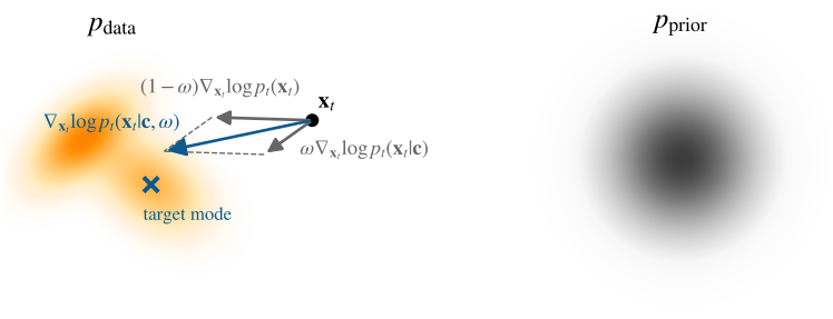
Classifier-free guidance (CFG) (Ho and Salimans 2021) removes the need for a separately trained classifier by expressing the classifier-guidance direction through conditional and unconditional scores. Bayes’ rule gives \[\begin{align} \nabla_{{\mathbf{x}}_t}\log p_t({\mathbf{c}}|{\mathbf{x}}_t) = \nabla_{{\mathbf{x}}_t}\log p_t({\mathbf{x}}_t|{\mathbf{c}}) - \nabla_{{\mathbf{x}}_t}\log p_t({\mathbf{x}}_t). \end{align}\] Substituting this identity into Equation \(\eqref{eq:cg_omega}\) gives the oracle CFG field \[\begin{align} \label{eq:cfg-model} {\mathbf{s}}^{\mathrm{CFG}}({\mathbf{x}}_t,t,{\mathbf{c}};\omega) &:= \nabla_{{\mathbf{x}}_t}\log p_t({\mathbf{x}}_t) + \omega \left( \nabla_{{\mathbf{x}}_t}\log p_t({\mathbf{x}}_t|{\mathbf{c}}) - \nabla_{{\mathbf{x}}_t}\log p_t({\mathbf{x}}_t) \right) \nonumber\\ &= \omega \underbrace{\nabla_{{\mathbf{x}}_t}\log p_t({\mathbf{x}}_t|{\mathbf{c}})}_{\text{conditional score}} + (1-\omega) \underbrace{\nabla_{{\mathbf{x}}_t}\log p_t({\mathbf{x}}_t)}_{\text{unconditional score}}. \end{align}\] With exact scores, Equation \(\eqref{eq:cfg-model}\) is algebraically the same guided field as Equation \(\eqref{eq:cg_omega}\). At \(\omega=1\), it reduces to the exact conditional score. For other guidance strengths, its fixed-time tilted-density interpretation should be distinguished from the marginals generated by the guided dynamics, as discussed in Section 1.4.2.

The hyperparameter \(\omega\) again plays a critical role in controlling the influence of the conditioning information (we take \(\omega \ge 0\)):

• At \(\omega = 0\), the model behaves as an unconditional diffusion model, completely ignoring the conditioning.

• At \(\omega = 1\), the model uses the conditional score without additional guidance.

• For \(\omega > 1\), the model places more emphasis on the conditional score and less on the unconditional score, strengthening alignment with \({\mathbf{c}}\) but typically reducing diversity.

Training and Sampling of CFG

Joint Training of Unconditional and Conditional Diffusion Models via CFG.

CFG requires a diffusion model trained to support both conditional and unconditional predictions. Rather than training two separate models, CFG uses a single model \({\mathbf{s}}_{\bm{\phi}}({\mathbf{x}}_t,t,{\mathbf{c}})\) and randomly replaces the conditioning input by a null token \(\emptyset\) during training:

• with the null input, the model learns the unconditional prediction \({\mathbf{s}}_{\bm{\phi}}({\mathbf{x}}_t,t,\emptyset)\);

• with the original condition, it learns the conditional prediction \({\mathbf{s}}_{\bm{\phi}}({\mathbf{x}}_t,t,{\mathbf{c}})\).

The null condition is used with probability \(p_\mathrm{uncond}\), a user-specified condition-dropout probability. The full training procedure is shown in Algorithm (CFG for Cond. DM), alongside standard unconditional training in Algorithm (Uncond. DM). The guidance weight \(\omega\) is introduced only at sampling time and is not part of this training objective.

Conditioned Sampling with CFG.

Once the model \({\mathbf{s}}_{\bm{\phi}^\times}({\mathbf{x}}_t,t,{\mathbf{c}})\) is trained using Algorithm (CFG for Cond. DM), CFG forms the learned guided field \[\begin{align} \label{eq:cfg-model-nn} {\mathbf{s}}_{\mathrm{model}}^{\mathrm{CFG}}({\mathbf{x}}_t,t,{\mathbf{c}};\omega) &:= \omega \underbrace{{\mathbf{s}}_{\bm{\phi}^\times}({\mathbf{x}}_t,t,{\mathbf{c}})}_{\text{conditional score estimate}} + (1-\omega) \underbrace{{\mathbf{s}}_{\bm{\phi}^\times}({\mathbf{x}}_t,t,\emptyset)}_{\text{unconditional score estimate}} \nonumber\\ &\approx {\mathbf{s}}^{\mathrm{CFG}}({\mathbf{x}}_t,t,{\mathbf{c}};\omega). \end{align}\] During sampling, the unconditional score estimate in the reverse-time SDE or PF-ODE is replaced by \({\mathbf{s}}_{\mathrm{model}}^{\mathrm{CFG}}\). Thus CFG defines a modified sampling field by combining the learned conditional and unconditional score estimates.

This formulation enables controllable generation by adjusting \(\omega\), providing a simple post-training trade-off between conditioning strength and sample diversity without requiring a separately trained classifier or unconditional diffusion model.

Training-Free Guidance

Training-free guidance modifies the sampling dynamics of a fixed pre-trained diffusion model using an external condition, loss, or measurement objective, without retraining the diffusion model itself. The Bayes decomposition in Equation \(\eqref{eq:guidance_bayes}\) provides a useful motivation in score space: guidance adds a condition-dependent direction to the unconditional score. In practice, a task-specific loss can be used to construct corrections either to the predicted clean sample or to the score used during sampling.

We first introduce these two general forms in Section 1.4.1. We then ask what distribution such surrogate-guided dynamics actually generate in Section 1.4.2, before turning to representative training-free approaches for inverse problems in Section 1.4.3.

Setup and Notations.

Let \({\mathbf{c}}\) denote a conditioning variable. We assume access to a pre-trained diffusion model \({\mathbf{s}}_{\bm{\phi}^\times}({\mathbf{x}}_t,t)\) expressed in score prediction⁴. In addition, suppose we are given a task loss \[\ell(\cdot,{\mathbf{c}})\colon\mathbb{R}^D\to\mathbb{R}\] that measures disagreement with the desired condition, so that smaller \(\ell({\mathbf{x}},{\mathbf{c}})\) indicates better agreement. Examples include a perceptual distance to a reference target, or a feature-space distance or negative similarity derived from a pre-trained representation such as CLIP (Radford et al. 2021).

Consider the standard linear–Gaussian forward noising kernel \[p_t(\cdot|{\mathbf{x}}_0) := \mathcal N\bigl(\cdot;\alpha_t{\mathbf{x}}_0,\sigma_t^2{\mathbf{I}}\bigr).\] We borrow the DDIM update introduced later in Equation in Chapter 9 as a concrete example: \[\begin{align} \label{eq:ddim-update-clean-noise-score} {\mathbf{x}}_{t\rightarrow t-1} = \alpha_{t-1} \underbrace{\hat{{\mathbf{x}}}_0({\mathbf{x}}_t)}_{\text{in data space}} - \sigma_{t-1}\sigma_t \underbrace{\hat{{\mathbf{s}}}({\mathbf{x}}_t)}_{\text{in noise space}}, \end{align}\] where \(\hat{{\mathbf{x}}}_0({\mathbf{x}}_t):={\mathbf{x}}_{\bm{\phi}^\times}({\mathbf{x}}_t,t)\) is the clean \({\mathbf{x}}\)-prediction and \(\hat{{\mathbf{s}}}({\mathbf{x}}_t):={\mathbf{s}}_{\bm{\phi}^\times}({\mathbf{x}}_t,t)\) is the score prediction at noise level \(t\).

Conceptual Framework for Training-Free Guidance

A common strategy is to use gradients of the task loss to modify either the predicted clean sample or the score term in the sampling update. To distinguish these two operations, define the data-space direction \[\mathcal G_t^{\mathrm{data}}({\mathbf{x}}_t,{\mathbf{c}}) := - \left. \nabla_{{\mathbf{x}}_0}\ell({\mathbf{x}}_0,{\mathbf{c}}) \right|_{{\mathbf{x}}_0=\hat{{\mathbf{x}}}_0({\mathbf{x}}_t)}.\] For the noise-space correction, we reuse the guidance direction introduced in the Prologue, \[\mathcal G_t({\mathbf{x}}_t,{\mathbf{c}}) := \nabla_{{\mathbf{x}}_t}\log{\mathbf{h}}_t({\mathbf{x}}_t;{\mathbf{c}}),\] for a positive guidance potential \({\mathbf{h}}_t\), specified below.

Using the DDIM update in Equation \(\eqref{eq:ddim-update-clean-noise-score}\), the two corrections can be written compactly as \[\begin{align} \label{eq:ddim-update-clean-noise-guide} \begin{aligned} {\mathbf{x}}_{t\rightarrow t-1} = \alpha_{t-1} \underbrace{\left( \hat{{\mathbf{x}}}_0({\mathbf{x}}_t) + {\color{orange} \eta_t^{\text{data}} \mathcal G_t^{\text{data}}({\mathbf{x}}_t,{\mathbf{c}})} \right)}_{\text{A. data space}} - \sigma_{t-1}\sigma_t \underbrace{\left( \hat{{\mathbf{s}}}({\mathbf{x}}_t) + {\color{orange} \eta_t^{\text{latent}} \mathcal G_t({\mathbf{x}}_t,{\mathbf{c}})} \right)}_{\text{B. noise space}}, \end{aligned} \end{align}\] where \(\eta_t^{\text{data}},\eta_t^{\text{latent}}\geq0\) control the strengths of the data-space and noise-space corrections, respectively.

A. Guidance in Data Space.

The data-space correction directly improves the current clean estimate by taking a local step that decreases the task loss: \[\hat{{\mathbf{x}}}_0({\mathbf{x}}_t) \;\longmapsto\; \hat{{\mathbf{x}}}_0({\mathbf{x}}_t) + \eta_t^{\text{data}} \mathcal G_t^{\text{data}}({\mathbf{x}}_t,{\mathbf{c}}).\] Thus the clean prediction is first moved toward better agreement with the condition and then used in the subsequent sampling update. This correction can also be applied repeatedly when multiple optimization steps are desired.

Representative examples include MGPD (He et al. 2023) and UGD (Bansal et al. 2023).

B. Guidance in Noise Space.

A closely related strategy applies guidance directly to the score used during sampling. Following the potential view introduced in Section 1.1, a common construction evaluates the task loss on the current denoised estimate and chooses \[{\mathbf{h}}_t({\mathbf{x}}_t;{\mathbf{c}}) := \exp\!\left( -\tau\,\ell\bigl(\hat{{\mathbf{x}}}_0({\mathbf{x}}_t),{\mathbf{c}}\bigr) \right), \qquad \tau>0.\] By the definition of \(\mathcal G_t\) above, this gives \[\begin{align*} \mathcal G_t({\mathbf{x}}_t,{\mathbf{c}}) = \nabla_{{\mathbf{x}}_t}\log{\mathbf{h}}_t({\mathbf{x}}_t;{\mathbf{c}}) = -\tau \nabla_{{\mathbf{x}}_t} \ell\bigl(\hat{{\mathbf{x}}}_0({\mathbf{x}}_t),{\mathbf{c}}\bigr). \end{align*}\] Accordingly, the score term in Equation \(\eqref{eq:ddim-update-clean-noise-guide}\) becomes \[\hat{{\mathbf{s}}}({\mathbf{x}}_t) + \eta_t^{\text{latent}} \mathcal G_t({\mathbf{x}}_t,{\mathbf{c}}).\] Comparing this practical update with the population-level construction in Equation \(\eqref{eq:generic-guided-score}\), \(\eta_t^{\text{latent}}\) plays the role of the generic guidance strength \(w_t\), while \(\hat{{\mathbf{s}}}({\mathbf{x}}_t)\) replaces the exact unconditional score by its learned estimate.

When \({\mathbf{h}}_t({\mathbf{x}}_t;{\mathbf{c}})\) is proportional to the true conditional likelihood \(p_t({\mathbf{c}}|{\mathbf{x}}_t)\) up to a factor independent of \({\mathbf{x}}_t\), \(\mathcal G_t({\mathbf{x}}_t,{\mathbf{c}})\) recovers the Bayes guidance direction \(\nabla_{{\mathbf{x}}_t}\log p_t({\mathbf{c}}|{\mathbf{x}}_t)\). For a generic task loss, \(\mathcal G_t\) instead defines a surrogate guidance direction.

Evaluating \(\mathcal G_t\) requires differentiating through the \({\mathbf{x}}\)-prediction: \[\mathcal G_t({\mathbf{x}}_t,{\mathbf{c}}) = -\tau \left[ \nabla_{{\mathbf{x}}_t}\hat{{\mathbf{x}}}_0({\mathbf{x}}_t) \right]^\top \left. \nabla_{{\mathbf{x}}_0}\ell({\mathbf{x}}_0,{\mathbf{c}}) \right|_{{\mathbf{x}}_0=\hat{{\mathbf{x}}}_0({\mathbf{x}}_t)},\] which may incur substantial computational cost in practice.

Representative examples include (Yu et al. 2023; Chung et al. 2022; Bansal et al. 2023).

The constructions above specify how guidance modifies each sampling step. They do not, by themselves, determine the marginal distributions obtained after these modified dynamics are integrated across all noise levels. We clarify this distinction next.

What Distribution Does Guided Sampling Produce?

The potential view above has an exact fixed-time density interpretation at the population level. In particular, replacing the learned unconditional score estimate \(\hat{{\mathbf{s}}}\) by the exact score, a positive potential \({\mathbf{h}}_t({\mathbf{x}};{\mathbf{c}})\) and guidance strength \(w_t\geq0\) define the ideal guided field \[\nabla_{{\mathbf{x}}}\log p_t({\mathbf{x}}) + w_t\nabla_{{\mathbf{x}}}\log{\mathbf{h}}_t({\mathbf{x}};{\mathbf{c}}).\] At each fixed \(t\), this is the score of \[\begin{align} \widetilde p_t^{\mathrm{tilt}}({\mathbf{x}}|{\mathbf{c}}) = \frac{1}{Z_t({\mathbf{c}})} p_t({\mathbf{x}}){\mathbf{h}}_t({\mathbf{x}};{\mathbf{c}})^{w_t}, \qquad Z_t({\mathbf{c}}) = \int p_t({\mathbf{x}}){\mathbf{h}}_t({\mathbf{x}};{\mathbf{c}})^{w_t}\,\mathop{}\!\mathrm{d}{\mathbf{x}}, \label{eq:guided-fixed-time-tilt} \end{align}\] provided \(0<Z_t({\mathbf{c}})<\infty\). The learned field used in practice approximates this ideal construction through the learned score estimate \(\hat{{\mathbf{s}}}({\mathbf{x}}_t)\).

For the loss-based construction above, \[{\mathbf{h}}_t({\mathbf{x}}_t;{\mathbf{c}}) = \exp\!\left[ -\tau\ell\bigl(\hat{{\mathbf{x}}}_0({\mathbf{x}}_t),{\mathbf{c}}\bigr) \right],\] and \(\eta_t^{\mathrm{latent}}\) plays the role of \(w_t\).

This fixed-time identity does not determine the distribution generated after the guided dynamics are integrated across noise levels. Consequently, for a generic loss and guidance schedule, solving the guided PF-ODE from \(T\) to \(0\) does not in general produce samples distributed according to \(\widetilde p_0^{\mathrm{tilt}}(\cdot|{\mathbf{c}})\).

The reason is cross-time consistency: densities at different noise levels cannot be chosen independently. For \(\{\widetilde p_t^{\mathrm{tilt}}\}_t\) to form the marginal path associated with the same forward diffusion, they must also satisfy the corresponding Fokker-Planck equation: \[\partial_t \widetilde p_t^{\mathrm{tilt}} + \nabla_{{\mathbf{x}}} \cdot \bigl(f(t){\mathbf{x}}\widetilde p_t^{\mathrm{tilt}}\bigr) - \frac{1}{2}g^2(t) \Delta_{{\mathbf{x}}}\widetilde p_t^{\mathrm{tilt}} = 0.\] When this condition holds, the corresponding PF-ODE \[\frac{\mathop{}\!\mathrm{d}{\mathbf{x}}(t)}{\mathop{}\!\mathrm{d}t} = f(t){\mathbf{x}}(t) - \frac{1}{2}g^2(t) \nabla_{{\mathbf{x}}}\log \widetilde p_t^{\mathrm{tilt}}\left({\mathbf{x}}(t)|{\mathbf{c}}\right)\] has \(\widetilde p_t^{\mathrm{tilt}}\) as its marginal path when initialized from the corresponding terminal distribution \(\widetilde p_T^{\mathrm{tilt}}(\cdot|{\mathbf{c}})\).

The compatibility condition can be checked directly. Substituting Equation \(\eqref{eq:guided-fixed-time-tilt}\) into the Fokker-Planck equation and using the fact that \(p_t\) itself satisfies the same equation gives \[\begin{align*} & \partial_t \widetilde p_t^{\mathrm{tilt}} + \nabla_{{\mathbf{x}}} \cdot \bigl(f(t){\mathbf{x}}\widetilde p_t^{\mathrm{tilt}}\bigr) - \frac{1}{2}g^2(t) \Delta_{{\mathbf{x}}}\widetilde p_t^{\mathrm{tilt}} \\ &= \widetilde p_t^{\mathrm{tilt}} \Bigg[ \partial_t \log \bigl({\mathbf{h}}_t^{ w_t}\bigr) + f(t){\mathbf{x}}\cdot \nabla_{{\mathbf{x}}}\log \bigl({\mathbf{h}}_t^{ w_t}\bigr) - g^2(t) \nabla_{{\mathbf{x}}}\log p_t \cdot \nabla_{{\mathbf{x}}}\log \bigl({\mathbf{h}}_t^{ w_t}\bigr) \\[-2pt] &\hspace{3.4cm} - \frac{1}{2}g^2(t) \left( \Delta_{{\mathbf{x}}}\log \bigl({\mathbf{h}}_t^{ w_t}\bigr) + \left\| \nabla_{{\mathbf{x}}}\log \bigl({\mathbf{h}}_t^{ w_t}\bigr) \right\|^2 \right) - \frac{Z_t'}{Z_t} \Bigg], \end{align*}\] where the arguments \(({\mathbf{x}};{\mathbf{c}})\) are suppressed for readability. Thus, the tilted family is a valid marginal path only when the bracketed quantity vanishes. A generic task loss and guidance schedule need not satisfy this condition. The mismatch can therefore remain even with exact score evaluation and exact ODE integration: it comes from the guided dynamics themselves rather than from numerical discretization. This is an instance of the broader Fokker-Planck consistency requirement discussed in (Lai et al. 2023).

Two simple cases clarify the distinction. When \(w_t\equiv0\), the tilt vanishes and the original unconditional path \(p_t\) is recovered. For exact classifier guidance, under the standard setting where the forward diffusion corrupts \({\mathbf{x}}\) while leaving \({\mathbf{c}}\) fixed, \[{\mathbf{h}}_t({\mathbf{x}};{\mathbf{c}}) = p_t({\mathbf{c}}|{\mathbf{x}}), \qquad w_t\equiv1.\] Bayes’ rule then gives \[\widetilde p_t^{\mathrm{tilt}}({\mathbf{x}}|{\mathbf{c}}) = p_t({\mathbf{x}}|{\mathbf{c}}),\] so the tilted family is exactly the conditional marginal path. This explains the special role of guidance weight \(1\) for the oracle classifier likelihood.

For a general guidance strength, for example \[p_t({\mathbf{x}}) p_t({\mathbf{c}}|{\mathbf{x}})^\omega,\] the expression still defines a valid fixed-time tilted density whenever it is normalizable, but it is not generally guaranteed to describe the marginals of the guided sampler. Special choices may satisfy the required compatibility condition, so \(\omega\neq1\) alone does not imply inconsistency.

Correction-based approaches such as Feynman-Kac Correctors (Skreta et al. 2025) explicitly account for this cross-time mismatch when the goal is to follow a prescribed sequence of tilted distributions more faithfully.

Examples of Training-Free Approaches to Inverse Problems

The principle introduced in Section 1.4.1 has important applications in inverse problems. We begin with an overview of the background and then provide several concrete examples illustrating how to leverage pre-trained diffusion models for inference-time inverse problem solving.

Background on Inverse Problems.

Let \(\mathcal A\) denote a known forward operator, possibly nonlinear, and suppose that \[\begin{align} \label{eq:inverse_problem} {\mathbf{y}} = \mathcal A({\mathbf{x}}_0) + \sigma_{{\mathbf{y}}}{\mathbf{z}}, \qquad {\mathbf{z}}\sim\mathcal N(\bm 0,{\mathbf{I}}). \end{align}\] The Bayesian objective is to characterize the posterior \(p_0({\mathbf{x}}_0|{\mathbf{y}})\), which combines the measurement model with prior knowledge about plausible clean signals. Blind inverse problems extend this setting by treating unknown parameters of \(\mathcal A\) as additional quantities to infer.

Classical inverse-problem methods commonly combine a data-fidelity term with an analytical or hand-designed prior in a variational or Bayesian formulation. Supervised restoration methods may instead learn a direct mapping from measurements to clean signals using paired data. Pre-trained diffusion models provide a third route: a learned prior over clean data can be reused across measurement operators, with measurement information introduced only at inference time.

Pre-Trained Diffusion Models as Inverse Problem Solvers.

For the measurement model above, Bayes’ rule gives \[\begin{align} \nabla_{{\mathbf{x}}_t}\log p_t({\mathbf{x}}_t|{\mathbf{y}}) = \underbrace{\nabla_{{\mathbf{x}}_t}\log p_t({\mathbf{x}}_t)}_{\text{data score}} + \underbrace{\nabla_{{\mathbf{x}}_t}\log p_t({\mathbf{y}}|{\mathbf{x}}_t)}_{\text{measurement guidance}}. \label{eq:bayes_rule} \end{align}\] The data score can be supplied by a pre-trained diffusion model, whereas the measurement term is generally unavailable in closed form. Training-free inverse solvers therefore introduce measurement information during sampling, but they need not all do so in the same mathematical form.

A useful distinction is between two common strategies. Some methods directly enforce measurement consistency by modifying or projecting the intermediate sample. Others approximate the likelihood score \(\nabla_{{\mathbf{x}}_t}\log p_t({\mathbf{y}}|{\mathbf{x}}_t)\) and add it to the data score through Equation \(\eqref{eq:bayes_rule}\).

ILVR (Choi et al. 2021).

ILVR provides a simple example of the first strategy. Let \(\phi_N\) denote its linear low-pass operator. At each reverse step, one first samples an unconditional proposal \[{\mathbf{x}}_{t-1}' \sim p_{\bm\theta}({\mathbf{x}}_{t-1}'|{\mathbf{x}}_t)\] and noises the reference image to the same level, \[{\mathbf{y}}_{t-1} \sim p_{t-1}({\mathbf{y}}_{t-1}|{\mathbf{y}}).\] The proposal is then refined according to \[{\mathbf{x}}_{t-1} = \phi_N({\mathbf{y}}_{t-1}) + ({\mathbf{I}}-\phi_N){\mathbf{x}}_{t-1}'.\] Thus, the prescribed low-frequency component comes from the noised reference, while the complementary component comes from the unconditional diffusion proposal. This is a sample-space consistency correction rather than an explicit approximation of \(\nabla_{{\mathbf{x}}_t}\log p_t({\mathbf{y}}|{\mathbf{x}}_t)\).

Diffusion Posterior Sampling (DPS) (Chung et al. 2022).

For a known nonlinear forward operator \(\mathcal A\) with additive Gaussian measurement noise \(\sigma_{{\mathbf{y}}}>0\), Diffusion Posterior Sampling (DPS) approximates \[\begin{align} \label{eq:dps-score} \nabla_{{\mathbf{x}}_t}\log p_t({\mathbf{y}}|{\mathbf{x}}_t) \approx \nabla_{{\mathbf{x}}_t} \log p\bigl({\mathbf{y}}|X_0=\hat{\mathbf{x}}_0({\mathbf{x}}_t)\bigr), \end{align}\] where \(\hat{\mathbf{x}}_0({\mathbf{x}}_t):=\mathbb{E}[{\mathbf{x}}_0|{\mathbf{x}}_t]\) is the posterior mean of the clean sample given \({\mathbf{x}}_t\), typically estimated from the pre-trained diffusion model using Tweedie’s formula (Equation in Chapter 3).

This plug-in approximation replaces the posterior average of the measurement likelihood by its value at the posterior mean: \[\begin{align*} p_t({\mathbf{y}}|{\mathbf{x}}_t) &= \int p_t({\mathbf{y}}|{\mathbf{x}}_t, {\mathbf{x}}_0) p({\mathbf{x}}_0|{\mathbf{x}}_t) \mathrm{d}{\mathbf{x}}_0 \\ &= \int p_t({\mathbf{y}}|{\mathbf{x}}_0) p({\mathbf{x}}_0|{\mathbf{x}}_t) \mathrm{d}{\mathbf{x}}_0 \approx p_t\bigl({\mathbf{y}}|X_0=\hat{\mathbf{x}}_0({\mathbf{x}}_t)\bigr), \end{align*}\] where we have used that \({\mathbf{y}}\) depends only on \({\mathbf{x}}_0\) (not on \({\mathbf{x}}_t\)) given \({\mathbf{x}}_0\), and the approximation holds under the assumption that the posterior \(p({\mathbf{x}}_0|{\mathbf{x}}_t)\) is tightly peaked around its mean.

Since \[p_t\bigl({\mathbf{y}}|X_0 = \hat{\mathbf{x}}_0({\mathbf{x}}_t)\bigr) = \mathcal{N}\bigl({\mathbf{y}}; \mathcal{A}(\hat{\mathbf{x}}_0({\mathbf{x}}_t)), \sigma_{{\mathbf{y}}}^2 {\mathbf{I}}\bigr),\] we compute \[\begin{align*} \nabla_{{\mathbf{x}}_t} \log p_t({\mathbf{y}}|{\mathbf{x}}_t) &\approx \nabla_{{\mathbf{x}}_t} \log \mathcal{N}\bigl({\mathbf{y}}; \mathcal{A}(\hat{\mathbf{x}}_0), \sigma_{{\mathbf{y}}}^2 {\mathbf{I}}\bigr) \\ &= -\frac{1}{2\sigma_{{\mathbf{y}}}^2} \nabla_{{\mathbf{x}}_t} \bigl\| {\mathbf{y}}- \mathcal{A}(\hat{\mathbf{x}}_0) \bigr\|^2 \quad \\ &= \frac{1}{\sigma_{{\mathbf{y}}}^2} \left[ \mathcal{J}_{\mathcal{A}}\big(\hat{\mathbf{x}}_0({\mathbf{x}}_t)\big) \cdot \nabla_{{\mathbf{x}}_t} \hat{\mathbf{x}}_0({\mathbf{x}}_t) \right]^\top \bigl( {\mathbf{y}}- \mathcal{A}\big(\hat{\mathbf{x}}_0({\mathbf{x}}_t)\big) \bigr), \end{align*}\] where \(\mathcal{J}_{\mathcal{A}}\big(\hat{\mathbf{x}}_0({\mathbf{x}}_t)\big) := \nabla_{{\mathbf{x}}_0} \mathcal{A}({\mathbf{x}}) \big|_{{\mathbf{x}}= \hat{\mathbf{x}}_0({\mathbf{x}}_t)}\) denotes the Jacobian of the forward operator with respect to its input. This formula propagates the gradient through the score approximation pipeline, reflecting how the measurement likelihood changes with respect to perturbations in the noisy sample \({\mathbf{x}}_t\).

For linear inverse problems, this further simplifies to: \[\begin{align*} \nabla_{{\mathbf{x}}_t} \log p_t({\mathbf{y}}| {\mathbf{x}}_t) \approx \frac{1}{\sigma_{{\mathbf{y}}}^2} \,\, \left[ {\mathbf{A}}\cdot \nabla_{{\mathbf{x}}_t} \hat{\mathbf{x}}_0({\mathbf{x}}_t) \right]^\top \left({\mathbf{y}}- {\mathbf{A}}(\hat{\mathbf{x}}_0({\mathbf{x}}_t))\right). \end{align*}\]

A large body of work explores diffusion-based inverse problem solvers by proposing various approximations for \(\nabla_{{\mathbf{x}}_t} \log p_t({\mathbf{y}}| {\mathbf{x}}_t)\). For a comprehensive overview, we refer readers to the survey by Daras et al. (2024).

A Related Supervised Iterative-Restoration Viewpoint and Its Connection to the PF-ODE.

The discussion above solves inverse problems by combining a pre-trained diffusion prior with the Bayes-rule decomposition in Equation \(\eqref{eq:bayes_rule}\). More specifically, these methods use the score of the prior distribution together with the measurement model to guide the reconstruction process. At the same time, they also reflect a broader idea: instead of recovering the clean signal in one step, they gradually improve a corrupted input through many small updates. A similar high-level strategy also appears in supervised image restoration, but from a different starting point. Rather than using a pre-trained score model as a prior, these methods learn the refinement procedure directly from paired corrupted and clean examples.

A representative example is InDI (Delbracio and Milanfar 2023). Unlike the Bayes-rule-based approaches above, InDI begins with paired data \(({\mathbf{y}},{\mathbf{x}}_0)\), where \({\mathbf{y}}\) is a corrupted observation and \({\mathbf{x}}_0\) is the corresponding clean target. Importantly, it does not assume in general that the corruption from \({\mathbf{x}}_0\) to \({\mathbf{y}}\) is known analytically or that it is Gaussian.

The basic idea is to connect the two endpoints by the interpolation path \[{\mathbf{x}}_t=(1-t){\mathbf{x}}_0+t{\mathbf{y}},\qquad t\in[0,1].\] This path should be understood only as a convenient trajectory from the clean target to the corrupted observation. It is not a Gaussian noising process in general. Along this path, for any \(0\le s\le t\), one has the exact relation \[{\mathbf{x}}_s=\Bigl(1-\frac{s}{t}\Bigr){\mathbf{x}}_0+\frac{s}{t}{\mathbf{x}}_t.\] Taking conditional expectation given \({\mathbf{x}}_t\) yields \[\mathbb E[{\mathbf{x}}_s|{\mathbf{x}}_t] = \Bigl(1-\frac{s}{t}\Bigr)\mathbb E[{\mathbf{x}}_0|{\mathbf{x}}_t] + \frac{s}{t}{\mathbf{x}}_t.\] This shows that, to move from the current state \({\mathbf{x}}_t\) to a slightly less degraded state, it is enough to predict the clean target from \({\mathbf{x}}_t\).

Based on this idea, one trains a time-conditioned predictor \({\mathbf{F}}_{{\bm{\phi}}}({\mathbf{x}}_t,t)\) from paired examples by minimizing the regression objective \[\min_{{\bm{\phi}}}\; \mathbb E_{({\mathbf{x}}_0,{\mathbf{y}})\sim p({\mathbf{x}}_0,{\mathbf{y}}), t\sim p(t)} \Bigl\| {\mathbf{F}}_{{\bm{\phi}}}\bigl((1-t){\mathbf{x}}_0+t{\mathbf{y}}, t\bigr)-{\mathbf{x}}_0 \Bigr\|_2^2,\] where \(p({\mathbf{x}}_0,{\mathbf{y}})\) denotes the joint distribution of data pairs consisting of a clean target \({\mathbf{x}}_0\) and its corrupted observation \({\mathbf{y}}\), and \(p(t)\) specifies how the interpolation time is sampled during training. That is, \({\mathbf{F}}_{{\bm{\phi}}}\) is trained to predict the clean target from an intermediate degraded state along the interpolation path. For this squared-error loss, the Bayes-optimal predictor is the conditional expectation \[{\mathbf{F}}^*({\mathbf{x}}_t,t)=\mathbb E[{\mathbf{x}}_0|{\mathbf{x}}_t].\] Therefore, if the model class is sufficiently expressive and the optimization is successful, the learned predictor approximates the average clean target associated with the intermediate state \({\mathbf{x}}_t\) at time \(t\). In this sense, the training objective is similar in spirit to diffusion-model training: in both cases, one learns a time-conditioned regression from an intermediate corrupted state to a cleaner target. The difference is that diffusion models generate such training pairs synthetically from a prescribed forward corruption process, whereas here the endpoint pairs \(({\mathbf{y}},{\mathbf{x}}_0)\) come directly from supervised restoration data.

At inference time, one starts from \(\hat{{\mathbf{x}}}_1={\mathbf{y}}\) and repeatedly refines the estimate by \[\hat{{\mathbf{x}}}_{t-\Delta t} = \frac{\Delta t}{t}{\mathbf{F}}_{{\bm{\phi}}}(\hat{{\mathbf{x}}}_t,t) + \Bigl(1-\frac{\Delta t}{t}\Bigr)\hat{{\mathbf{x}}}_t.\] Hence, the final reconstruction is produced by gradual refinement rather than by a single direct prediction. In the continuous-time limit, this leads to InDI’s residual-flow ODE \[\frac{\mathop{}\!\mathrm{d}{\mathbf{x}}_t}{\mathop{}\!\mathrm{d}t} = \frac{{\mathbf{x}}_t-{\mathbf{F}}_{{\bm{\phi}}}({\mathbf{x}}_t,t)}{t}.\]

Now suppose we further specialize to the Gaussian denoising setting, where the corruption is assumed to take the known analytic form \[{\mathbf{y}}={\mathbf{x}}_0+\sigma{\bm{\epsilon}}, \qquad {\bm{\epsilon}}\sim\mathcal N(\bm 0,{\mathbf{I}}),\] with known noise level \(\sigma\). Under this specialization, InDI’s residual-flow ODE reduces exactly to the probability-flow ODE. Indeed, the interpolation path becomes \[{\mathbf{x}}_t=(1-t){\mathbf{x}}_0+t{\mathbf{y}} = {\mathbf{x}}_0+t\sigma{\bm{\epsilon}},\] which is precisely the standard diffusion form \[{\mathbf{x}}_t=\alpha_t{\mathbf{x}}_0+\sigma_t{\bm{\epsilon}}, \qquad\text{with}\qquad \alpha_t=1,\;\sigma_t=t\sigma.\] Therefore, the predictor \({\mathbf{F}}_{{\bm{\phi}}}({\mathbf{x}}_t,t)\approx \mathbb E[{\mathbf{x}}_0\mid {\mathbf{x}}_t]\) is now learning to denoise a Gaussian-corrupted intermediate state \({\mathbf{x}}_t\). In this case, the residual-flow ODE becomes \[\frac{\mathop{}\!\mathrm{d}{\mathbf{x}}_t}{\mathop{}\!\mathrm{d}t} = \frac{{\mathbf{x}}_t-\mathbb E[{\mathbf{x}}_0\mid {\mathbf{x}}_t]}{t} = -\dot{\sigma}_t\sigma_t\nabla_{{\mathbf{x}}_t}\log p_t({\mathbf{x}}_t),\] where the last equality follows from \(\sigma_t=t\sigma\) together with Tweedie’s formula, \[\mathbb E[{\mathbf{x}}_0\mid {\mathbf{x}}_t] = {\mathbf{x}}_t+\sigma_t^2\nabla_{{\mathbf{x}}_t}\log p_t({\mathbf{x}}_t).\] This is exactly the PF-ODE for this Gaussian denoising path, written in either denoiser form or score form. Thus, under the Gaussian denoising specialization, InDI suggests an alternative interpretation of diffusion modeling: one may view it as supervised denoiser learning on Gaussian-corrupted data, with the PF-ODE arising as the continuous-time limit of gradual refinement.

From Reinforcement Learning to Direct Preference Optimization for Model Alignment

In the pursuit of aligning generative models with human intent, the prevailing paradigm has been Reinforcement Learning from Human Feedback (RLHF). While effective, RLHF is a complex, multi-stage process that can be unstable. This section introduces Direct Preference Optimization (DPO) (Rafailov et al. 2023), a more streamlined and stable method that reaches the same goal without explicit reward modeling or reinforcement learning. We then outline its extension to diffusion models via Diffusion-DPO (Wallace et al. 2024).

The Motivation: Circumventing the Pitfalls of RLHF

The goal of alignment is to steer a base, pre-trained model (e.g., an SFT model) toward outputs that humans prefer. RLHF proceeds in three stages. First, supervised fine-tuning (SFT) trains a base model on prompt–response pairs. Second, reward modeling (RM) fits a model on preference data consisting of prompts \(\mathbf{c}\) and paired responses (a preferred “winner” \(\mathbf{x}_w\) and a dispreferred “loser” \(\mathbf{x}_l\)), learning a scalar \(r(\mathbf{c},\mathbf{x})\) with \(r(\mathbf{c},\mathbf{x}_w)>r(\mathbf{c},\mathbf{x}_l)\). Third, RL fine-tuning optimizes the SFT model (policy \(\pi\)⁵) with an algorithm such as PPO (Schulman et al. 2017), maximizing expected reward from \(r\) while regularizing by a KL penalty that keeps \(\pi\) close to the reference/SFT distribution.

Despite its impact, this pipeline suffers from drawbacks: the RL stage is unstable and computationally expensive because it is on-policy—each update requires freshly generated samples from the current model; it also requires training and hosting multiple large models (SFT, reward, and sometimes a value model); and it optimizes only a proxy for human preferences, so flaws in the reward model can be exploited. This motivates a central question:

Direct Preference Optimization (DPO) streamlines alignment by replacing the multi-stage RLHF pipeline with a single, supervised-style step. Instead of training a separate reward model and running unstable RL algorithms like PPO, DPO directly fits the policy to preference pairs using a simple logistic loss, while staying close to a fixed reference model. The key insight is that the KL-regularized RLHF objective can be rewritten so that the log-likelihood ratio between the policy and the reference acts as an implicit reward. This preserves the same regularization toward the reference policy but avoids costly rollouts and explicit reward modeling.

In Section 1.5.2, we briefly review the RLHF pipeline and its reliance on large reward models and RL fine-tuning. In Section 1.5.3, we present DPO, originally proposed for language models, which circumvents reward model training and simplifies alignment fine-tuning. Finally, in Section 1.5.4, we extend this idea to diffusion models, introducing Diffusion-DPO as a practical and stable alignment method in the generative modeling setting.

RLHF: Bradley-Terry View

Short Introduction to RLHF.

RLHF begins with a learned judge: a reward model \(r_{\bm\psi}\) that assigns a scalar preference score to candidate responses for the same prompt \(\mathbf c\). The dataset \(\mathcal D\) consists of pairs \((\tilde{\mathbf x},\mathbf x)\) annotated with a label \(y\) indicating whether \(\tilde{\mathbf x}\) is preferred over \(\mathbf x\). The label can be binary \(y\in\{0,1\}\) or a soft value \(y\in[0,1]\) obtained by aggregating multiple raters. The training objective is a simple logistic loss \[\begin{align} \label{eq:rm-emp} \begin{aligned} \mathcal L_{\mathrm{RM}}(\bm\psi) = - \mathbb E_{(\mathbf c,\tilde{\mathbf x},\mathbf x,y)\sim\mathcal D} \Big[ y &\log \sigma \big(r_{\bm\psi}(\mathbf c,\tilde{\mathbf x})-r_{\bm\psi}(\mathbf c,\mathbf x)\big) \\ &+(1-y)\log \big(1-\sigma \big(r_{\bm\psi}(\mathbf c,\tilde{\mathbf x})-r_{\bm\psi}(\mathbf c,\mathbf x)\big)\big) \Big], \end{aligned} \end{align}\] where \(\sigma(u)=1/(1+e^{-u})\). In practice, preference pairs in \(\mathcal D\) may originate from various sources: curated responses, model snapshots at different checkpoints, or generations from a pre-trained conditional diffusion model. A standard convention is to store them in an ordered format \((\text{winner}, \text{loser})\). Under this convention we simply set \(y=1\), and Equation \(\eqref{eq:rm-emp}\) reduces to the special case (with \(\tilde{\mathbf{x}}= {\mathbf{x}}^w\) and \({\mathbf{x}}= {\mathbf{x}}^l\)): \[\begin{equation} \label{eq:rm-bt} \mathcal L_{\mathrm{RM}}(\bm\psi) = - \mathbb E_{(\mathbf c,\mathbf x_w,\mathbf x_l)\sim\mathcal D} \Big[\log \sigma \big(r_{\bm\psi}(\mathbf c,\mathbf x_w)-r_{\bm\psi}(\mathbf c,\mathbf x_l)\big)\Big]. \end{equation}\]

Bradley-Terry View and KL Connection.

It is standard to interpret \[p_{r_{\bm\psi}}(\tilde{\mathbf x}\succ \mathbf x|\mathbf c) := \sigma \big(r_{\bm\psi}(\mathbf c,\tilde{\mathbf x})-r_{\bm\psi}(\mathbf c,\mathbf x)\big)\] through the Bradley-Terry (BT) model (Bradley and Terry 1952), which converts two scalar scores into a win probability. This formulation highlights two key properties: (i) only the difference of scores matters (so \(r_{\bm\psi}(\mathbf c,\cdot)\) is shift-invariant), and (ii) the loss pushes the predicted winner’s score above the loser’s score. To see (ii) intuitively, consider one pair with label \(y\in\{0,1\}\) and define \[\Delta r := r_{\bm\psi}(\mathbf c,\tilde{\mathbf x})-r_{\bm\psi}(\mathbf c,\mathbf x), \quad p:=\sigma(\Delta r),\quad \sigma(u)=\tfrac{1}{1+e^{-u}}.\] The per-example logistic loss is \[\ell=-\big[y\log p+(1-y)\log(1-p)\big].\] Then \[\frac{\partial \ell}{\partial \Delta r}=\sigma(\Delta r)-y.\] Under gradient descent with step size \(\eta>0\), the score gap updates as \[\Delta r \leftarrow \Delta r-\eta\big(\sigma(\Delta r)-y\big).\] Hence, if \(y=1\) (“\(\tilde{\mathbf x}\) wins”), then \(\sigma(\Delta r)-1\le 0\), so \(\Delta r\) increases (winner up, loser down); if \(y=0\), \(\Delta r\) decreases.

Each per-example term in Equation \(\eqref{eq:rm-emp}\) can be viewed as the cross-entropy between the observed Bernoulli label and the model’s predicted win probability: \[-\big[y\log p_{r_{\bm\psi}}+(1-y)\log(1-p_{r_{\bm\psi}})\big] = \mathcal D_{\mathrm{KL}} \big(\mathrm{Bern}(y) \big\| \mathrm{Bern}(p_{r_{\bm\psi}})\big) + \mathcal H \big(\mathrm{Bern}(y)\big),\] where \(\mathcal H\) is the entropy of the target Bernoulli distribution. Averaging over the dataset \(\mathcal D\) gives \[\begin{align} \label{eq:reward_loss} \mathcal L_{\mathrm{RM}}(\bm\psi) = \mathbb E_{\mathcal D} \Big[\mathcal D_{\mathrm{KL}}\left(\mathrm{Bern}(y) \big\| \mathrm{Bern}(p_{r_{\bm\psi}})\right)\Big] + \underbrace{\mathbb E_{\mathcal D} \big[\mathcal H(\mathrm{Bern}(y))\big]}_{\text{independent of }\bm\psi}. \end{align}\] Thus, minimizing the logistic loss is equivalent to minimizing the KL divergence between the empirical Bernoulli distribution of human labels and the model’s predicted Bernoulli distribution. In the binary case (\(y\in\{0,1\}\)), this equivalence is exact; for soft labels (\(y\in[0,1]\)), the result holds up to an entropy constant offset. Intuitively, the reward model is trained to adjust its win probabilities until they align with the empirical human win rates observed in the dataset.

From this point onward, we adopt the most common convention where \(\mathcal D\) stores pairs in an ordered format: \(({\mathbf{x}}^w, {\mathbf{x}}^l, {\mathbf{c}}) \sim \mathcal D\). Under this convention, the label is always \(y=1\), and the loss simplifies to the ordered form given in Equation \(\eqref{eq:rm-bt}\), which we will use in the following discussion.

KL Regularized Policy Optimization (with Fixed Reward).

With the fitted reward \(r:=r_{\bm\psi^\times}\) trained via Equation \(\eqref{eq:rm-bt}\), and a conditional pre-trained diffusion model \(p_{\bm{\phi}^\times}(\mathbf x|\mathbf c)\), RLHF then adjusts a learnable policy \(\pi_{\bm\theta}(\mathbf x|\mathbf c)\), usually fine-tuned on top of \(p_{\bm{\phi}^\times}(\mathbf x|\mathbf c)\), toward higher-reward responses. At the same time, the policy is regularized to stay close to a reference model, taken as the pre-trained diffusion model \(\pi_{\mathrm{ref}}(\mathbf x|\mathbf c):=p_{\bm{\phi}^\times}(\mathbf x|\mathbf c)\), using a \(\mathcal{D}_{\mathrm{KL}}\) penalty: \[\begin{equation} \label{eq:rlhf-policy-correct} \max_{\bm\theta} \mathbb E_{\mathbf c\sim p(\mathbf c)} \Big[ \mathbb E_{\mathbf x\sim \pi_{\bm\theta}(\cdot|\mathbf c)}\big[r_{\bm\psi}(\mathbf c,\mathbf x)\big] -\beta \mathcal{D}_{\mathrm{KL}} \big(\pi_{\bm\theta}(\cdot|\mathbf c) \big\| \pi_{\mathrm{ref}}(\cdot|\mathbf c)\big) \Big], \end{equation}\] which makes the two forces explicit: seek samples the judge prefers, but stay close to the pre-trained reference.

We remark that the reward objective in Equation \(\eqref{eq:rm-bt}\) uses only labeled pairs and does not require that \(\mathcal D\) be generated by the reference model (i,e., the pre-trained conditional diffusion model). While not required, collecting pairs from models close to the intended policy can reduce distribution shift and make the learned reward more reliable in the region where it will be used.

In summary, RLHF proceeds in two stages: first fit the reward \(r^*\) by minimizing the loss in Equation \(\eqref{eq:rm-bt}\) (equivalently, the expected binary \(\mathcal{D}_{\mathrm{KL}}\) in Equation \(\eqref{eq:reward_loss}\)); then optimize the policy \(\pi^*\) by solving Equation \(\eqref{eq:rlhf-policy-correct}\).

DPO Framework

The Bridge from RLHF.

The KL-regularized policy objective in Equation \(\eqref{eq:rlhf-policy-correct}\) has a simple closed-form solution for each prompt \(\mathbf c\), given the fitted reward \(r := r_{\bm\psi^\times}\), expressed in the following energy-based form (Peters et al. 2010): \[\begin{equation} \label{eq:rlhf-closed-form} \pi^*(\mathbf x|\mathbf c) = \frac{1}{Z(\mathbf c)} \pi_{\mathrm{ref}}(\mathbf x|\mathbf c)\exp(r(\mathbf c,\mathbf x)/\beta), \end{equation}\] where \(\pi_{\mathrm{ref}}(\mathbf x|\mathbf c):=p_{\bm{\phi}^\times}(\mathbf x|\mathbf c)\), and \(Z(\mathbf c)\) is the partition function ensuring \(\int \pi^*(\mathbf x|\mathbf c) \mathop{}\!\mathrm{d}\mathbf x=1\).

For smaller \(\beta\), \(\exp(r/\beta)\) becomes sharper, so \(\pi^*\) concentrates on high reward regions: reward dominates, the policy moves farther from \(\pi_{\mathrm{ref}}\), diversity decreases, and training may become unstable or prone to reward hacking. For larger \(\beta\), \(\exp(r/\beta)\) flattens, keeping \(\pi^*\) closer to \(\pi_{\mathrm{ref}}\): the KL term dominates, updates are conservative, diversity follows the reference, but reward gains are limited.

Since our aim is to fine-tune the policy directly (without training a separate reward model), Equation \(\eqref{eq:rlhf-closed-form}\) lets us define an implicit reward from any policy. We introduce below:

Defining an Implicit Reward Motivated by Inverting Equation \(\eqref{eq:rlhf-closed-form}\).

Equation \(\eqref{eq:rlhf-closed-form}\) suggests an immediate inversion: for any policy \(\pi\) (with support contained in \(\pi_{\mathrm{ref}}\)), define \[\begin{equation} \label{eq:implicit-reward} r_{\pi}(\mathbf c,\mathbf x) = \beta \log\frac{\pi(\mathbf x|\mathbf c)}{\pi_{\mathrm{ref}}(\mathbf x|\mathbf c)} + \beta \log Z(\mathbf c). \end{equation}\] Then Equation \(\eqref{eq:rlhf-closed-form}\) holds with \(\pi\) in place of \(\pi^*\), i.e., \(\pi\) would be the optimizer of Equation \(\eqref{eq:rlhf-policy-correct}\) for the reward function \(r_{\pi}\). In this sense, \(r_{\pi}\) is an implicit (policy-induced) reward: it is identified up to the prompt-dependent constant \(\beta\log Z(\mathbf c)\), which vanishes in any pairwise comparison such as in the BT model: \[r_{\pi}(\mathbf c,\mathbf x_w)-r_{\pi}(\mathbf c,\mathbf x_l) = \beta\Big( \log\frac{\pi(\mathbf x_w|\mathbf c)}{\pi_{\mathrm{ref}}(\mathbf x_w|\mathbf c)} - \log\frac{\pi(\mathbf x_l|\mathbf c)}{\pi_{\mathrm{ref}}(\mathbf x_l|\mathbf c)} \Big).\] This cancellation is exactly what makes the constant irrelevant for preference learning and leads directly to the DPO loss on log-probability differences.

DPO’s Training Loss.

Plug the implicit reward Equation \(\eqref{eq:implicit-reward}\) into the BT model of Equation \(\eqref{eq:rm-bt}\) for a labeled pair \((\mathbf x_w,\mathbf x_l)\) under the same prompt \(\mathbf c\). The constants \(\log Z(\mathbf c)\) cancel between winner and loser, yielding a single logistic-loss objective on log-probability differences: \[\begin{align*} \mathcal L_{\mathrm{DPO}}(\bm\theta;\pi_{\mathrm{ref}}) &= -\mathbb E_{(\mathbf c,\mathbf x_w,\mathbf x_l)\sim\mathcal D} \left[ \log \sigma \Big( \beta\big( \log\frac{\pi_{\bm\theta}(\mathbf x_w|\mathbf c)}{\pi_{\mathrm{ref}}(\mathbf x_w|\mathbf c)} - \log\frac{\pi_{\bm\theta}(\mathbf x_l|\mathbf c)}{\pi_{\mathrm{ref}}(\mathbf x_l|\mathbf c)} \big) \Big) \right]. \end{align*}\] In words: DPO pushes up the (temperature-scaled) advantage of the winner over the loser, measured as the difference of log-likelihood improvements over the reference: \[-\log \sigma \left( \beta \bigl[ \text{log-ratio difference of } \tfrac{\pi_{\bm\theta}}{\pi_{\mathrm{ref}}} \text{ at } \mathbf x_w \text{ vs.\ } \mathbf x_l \bigr] \right).\] This achieves the goal of RLHF in a single, stable classification-style fine-tuning stage, without training an explicit reward model.

Diffusion-DPO

Throughout this subsection, we retain the policy notation from Section 1.5.3: \(\pi_{\bm\theta}\) and \(\pi_{\mathrm{ref}}\) denote the learned and reference diffusion policies, including their path and transition distributions, while \(p_t({\mathbf{x}}_t|{\mathbf{x}}_0)\) continues to denote the fixed forward noising process.

Why Naive DPO Fails for Diffusion Models?

Evaluating the sample likelihood \(\pi_{\bm{\theta}}(\mathbf x|\mathbf c)\) in diffusion models requires the instantaneous change-of-variables formula (divergence of the drift) of ODE solving (see Equation in Chapter 4)⁶, which is computationally intensive. Moreover, differentiating through the entire sampling trajectory can suffer from vanishing or exploding gradients. To avoid these issues, Diffusion-DPO works at the path level. We take the discrete-time diffusion model (e.g., DDPM) as an illustrative example; the continuous-time diffusion model is analogous.

Defining Pathwise Implicit Rewards.

Let a trajectory be \(\mathbf x_{0:T}:=(\mathbf x_T,\ldots,\mathbf x_0)\) under the reverse-time Markov chain with conditionals \(\pi(\mathbf x_{t-1}|\mathbf x_t,\mathbf c)\). Here, \(\mathbf x_T\) is the highest-noise state and \(\mathbf x_0\) is the clean output.

Human preferences are defined on the final output through \(r(\mathbf c,\mathbf x_0)\). Since \(\mathbf x_0\) is part of every diffusion trajectory, the reward itself does not need to change when we move to path space. The useful step is instead to regularize the entire reverse process. By the chain rule for KL divergence, the KL divergence between the full path distributions is at least as large as the KL divergence between their endpoint marginals. This motivates the pathwise objective \[\max_{{\bm{\theta}}}\mathbb E_{\mathbf c\sim p(\mathbf c)} \Big[ \mathbb E_{\mathbf x_{0:T}\sim\pi_{{\bm{\theta}}}(\cdot|\mathbf c)} \big[r(\mathbf c,\mathbf x_0)\big] -\beta \mathcal D_{\mathrm{KL}} \big( \pi_{{\bm{\theta}}}(\cdot|\mathbf c) \big\| \pi_{\mathrm{ref}}(\cdot|\mathbf c) \big) \Big],\] where \(\pi_{{\bm{\theta}}}(\cdot|\mathbf c)\) and \(\pi_{\mathrm{ref}}(\cdot|\mathbf c)\) denote the corresponding path distributions. The reward term is unchanged, while the KL penalty now also controls how the latent denoising trajectories deviate from the reference.

At the distributional level, assuming the normalizer is finite, the optimizer for each prompt \(\mathbf c\) has the energy-based form \[\begin{equation} \label{eq:path-closed-form} \pi^*(\mathbf x_{0:T}|\mathbf c) = \frac{1}{Z(\mathbf c)} \pi_{\mathrm{ref}}(\mathbf x_{0:T}|\mathbf c) \exp\big(r(\mathbf c,\mathbf x_0)/\beta\big). \end{equation}\] As in ordinary DPO, we can invert this relation and define the implicit path reward induced by any policy \(\pi\): \[R_{\pi}(\mathbf c,\mathbf x_{0:T}) := \beta\log \frac{\pi(\mathbf x_{0:T}|\mathbf c)} {\pi_{\mathrm{ref}}(\mathbf x_{0:T}|\mathbf c)} +\beta\log Z(\mathbf c).\] At the pathwise optimum, \(R_{\pi^*}(\mathbf c,\mathbf x_{0:T})=r(\mathbf c,\mathbf x_0)\). For a general policy, however, \(R_{\pi}\) may also depend on the latent trajectory. Since the preference data compare only the clean endpoints, we therefore average this implicit path reward over trajectories associated with each endpoint.

From Pathwise Implicit Rewards to DPO.

For a labeled endpoint pair \((\mathbf x_0^w,\mathbf x_0^l)\) under the same prompt \(\mathbf c\), the Bradley–Terry margin is obtained by comparing the conditional averages of their implicit path rewards: \[\begin{align} \label{eq:diffusion-dpo} \begin{aligned} \mathcal L_{\mathrm{Diff\text{-}DPO}}(\bm\theta;\pi_{\mathrm{ref}}) &:= - \mathbb E_{(\mathbf c,\mathbf x_0^w,\mathbf x_0^l)\sim\mathcal D} \left[\log \sigma \big(\Delta R(\mathbf c;\bm\theta)\big)\right], \quad \text{where}\\ \Delta R(\mathbf c;\bm\theta) &:= \underbrace{\mathbb E_{\mathbf x_{1:T}^w\sim \pi_{\bm\theta}(\cdot | \mathbf x_0^w,\mathbf c)} \Big[R_{\pi_{\bm\theta}} \big(\mathbf c,(\mathbf x_0^w,\mathbf x_{1:T}^w)\big)\Big]}_{\text{winner path expectation}} \\ &\quad\quad\quad- \underbrace{\mathbb E_{\mathbf x_{1:T}^l\sim \pi_{\bm\theta}(\cdot | \mathbf x_0^l,\mathbf c)} \Big[R_{\pi_{\bm\theta}} \big(\mathbf c,(\mathbf x_0^l,\mathbf x_{1:T}^l)\big)\Big]}_{\text{loser path expectation}}. \end{aligned} \end{align}\] Here, the expectation \(\mathbb E_{\mathbf x_{1:T}\sim\pi_{\bm\theta}(\cdot|\mathbf x_0,\mathbf c)}[\cdot]\) means: given a fixed endpoint \(\mathbf x_0\) (e.g., the winner \(\mathbf x_0^w\)) from the dataset, we take an expectation over latent denoising trajectories \(\mathbf x_{1:T}\) under the model-induced conditional path distribution (the posterior over reverse-time trajectories) that, with kernels \(\pi_{\bm\theta}(\mathbf x_{t-1}|\mathbf x_t,\mathbf c)\), could produce \(\mathbf x_0\). Since these intermediate states are unobserved, we average the path reward over all such trajectories.

However, Equation \(\eqref{eq:diffusion-dpo}\) is impractical for three practical reasons:

1. Endpoint Conditioning Induces an Intractable Path Posterior. The term \(\mathbb E_{\pi_{\bm\theta}(\mathbf x_{1:T}|\mathbf x_0,\mathbf c)}[\cdot]\) averages over reverse paths constrained to hit \(\mathbf x_0\), whereas the sampler runs \(\mathbf x_T \to \cdots \to \mathbf x_0\) without this constraint. Conditioning on the endpoint creates a diffusion-bridge posterior with generally no closed form and costly sampling.

2. Nested, \(\bm\theta\)-Coupled Expectations. The loss \(-\log\sigma(\Delta R(\mathbf c;\bm\theta))\) with \[\Delta R=\mathbb E_{\text{paths}|\mathbf x_0^w,\mathbf c}[R_{\pi_{\bm\theta}}] -\mathbb E_{\text{paths}|\mathbf x_0^l,\mathbf c}[R_{\pi_{\bm\theta}}]\] has both the path joint distribution and the integrand \(R_{\pi_{\bm\theta}}\) depending on \(\bm\theta\). Thus \(\nabla_{\bm\theta}\) must differentiate through the sampling distribution, leading to REINFORCE/pathwise couplings and high-variance gradients.

3. Long Chains, Large Sums, and Expensive Backpropagation. In \(R_{\pi_{\bm\theta}}(\mathbf c,\mathbf x_{0:T})\), computing \[\beta \left[\log \pi_{\bm\theta}(\mathbf x_{0:T}|\mathbf c) -\log \pi_{\mathrm{ref}}(\mathbf x_{0:T}|\mathbf c)\right]\] requires \(\mathcal O(T)\) per-step log-densities with \(T \sim 10^2\)–\(10^3\), for both policy \(\pi_{\bm\theta}\) and reference \(\pi_{\mathrm{ref}}\), and for both winner/loser paths. Backpropagating through these stochastic chains (or bridge samplers) is memory and compute heavy and can be unstable; repeating this over many samples per pair and across all triplets pushes training beyond practical budgets.

Toward a Tractable Surrogate for Equation \(\eqref{eq:diffusion-dpo}\).

To make this computable, we apply a key mathematical insight. By leveraging properties of diffusion models and applying Jensen’s inequality, we can optimize a tractable upper bound on this loss. This transforms the problem from evaluating an entire path’s likelihood to evaluating an expectation over the individual, single-step transitions within the path:

Because \(-\log\sigma(\cdot)\) is convex, Jensen’s inequality yields an upper bound by moving the inner expectations outside the nonlinear function: \[\begin{align*} \mathcal L_{\mathrm{Diff\text{-}DPO}}(\bm\theta;\pi_{\mathrm{ref}}) \le -\mathbb E_{(\mathbf c,\mathbf x_0^w,\mathbf x_0^l)\sim\mathcal D} \mathbb E_{\substack{\mathbf x^w_{1:T}\sim \pi_{\bm\theta}(\cdot | \mathbf x_0^w,\mathbf c)\\[1pt] \mathbf x^l_{1:T}\sim \pi_{\bm\theta}(\cdot | \mathbf x_0^l,\mathbf c)}} \left[ \log \sigma \Big( R_{\pi_{\bm\theta}}(\mathbf c,\mathbf x^w_{0:T}) - R_{\pi_{\bm\theta}}(\mathbf c,\mathbf x^l_{0:T}) \Big) \right]. \end{align*}\] Using the implicit-reward identity \(R_{\pi_{\bm\theta}}=\beta\log\frac{\pi_{\bm\theta}}{\pi_{\mathrm{ref}}}+\beta\log Z(\mathbf c)\) and cancellation of the constant between winner and loser, the bound becomes \[\begin{align} \label{eq:dpo-path-bound} \mathcal L_{\mathrm{Diff\text{-}DPO}}(\bm\theta;\pi_{\mathrm{ref}}) & \le -\mathbb E \left[ \log \sigma \Big( \beta\big( \log\frac{\pi_{\bm\theta}(\mathbf x^w_{0:T}| \mathbf c)}{\pi_{\mathrm{ref}}(\mathbf x^w_{0:T}| \mathbf c)} - \log\frac{\pi_{\bm\theta}(\mathbf x^l_{0:T}| \mathbf c)}{\pi_{\mathrm{ref}}(\mathbf x^l_{0:T}| \mathbf c)} \big) \Big) \right]. \end{align}\]

A Tractable Surrogate (Stepwise Form).

We now exploit the Markov property of the reverse process to decompose the upper bound of \(\mathcal L_{\mathrm{Diff\text{-}DPO}}\). This allows us to express the path-level preference as a sum of per-step contributions, converting the intractable pathwise loss into a tractable single-step estimator. The resulting form yields a DPO-style log-sigmoid loss whose inner margin reduces to a DSM-style MSE difference. Concretely, for the reverse chain, \[\begin{align*} \pi_{\bm\theta}(\mathbf x_{0:T}| \mathbf c) &=\pi_{\bm\theta}(\mathbf x_T| \mathbf c) \prod_{t=1}^{T} \pi_{\bm\theta}(\mathbf x_{t-1}| \mathbf x_t,\mathbf c), \\ \pi_{\mathrm{ref}}(\mathbf x_{0:T}| \mathbf c) &=\pi_{\mathrm{ref}}(\mathbf x_T| \mathbf c) \prod_{t=1}^{T} \pi_{\mathrm{ref}}(\mathbf x_{t-1}| \mathbf x_t,\mathbf c). \end{align*}\] Hence \[\frac{\pi_{\bm\theta}(\mathbf x_{0:T}| \mathbf c)}{\pi_{\mathrm{ref}}(\mathbf x_{0:T}| \mathbf c)} = \frac{\pi_{\bm\theta}(\mathbf x_T| \mathbf c)}{\pi_{\mathrm{ref}}(\mathbf x_T| \mathbf c)} \prod_{t=1}^{T} \frac{\pi_{\bm\theta}(\mathbf x_{t-1}| \mathbf x_t,\mathbf c)} {\pi_{\mathrm{ref}}(\mathbf x_{t-1}| \mathbf x_t,\mathbf c)}.\] If the prior at time \(T\) is the same for both models, \(\pi_{\bm\theta}(\mathbf x_T| \mathbf c)=\pi_{\mathrm{ref}}(\mathbf x_T| \mathbf c)\), then the first factor equals \(1\), and taking logs yields \[\log\frac{\pi_{\bm\theta}(\mathbf x_{0:T}| \mathbf c)}{\pi_{\mathrm{ref}}(\mathbf x_{0:T}| \mathbf c)} =\sum_{t=1}^{T} \log\frac{\pi_{\bm\theta}(\mathbf x_{t-1}| \mathbf x_t,\mathbf c)} {\pi_{\mathrm{ref}}(\mathbf x_{t-1}| \mathbf x_t,\mathbf c)}.\] It follows that the bound in Equation \(\eqref{eq:dpo-path-bound}\) can be written as \[\mathcal L_{\mathrm{Diff\text{-}DPO}}(\bm\theta;\pi_{\mathrm{ref}}) \le - \mathbb{E}\left[\log\sigma \Big(\beta \sum_{t=1}^T \Delta_t\Big)\right],\] where each per-step contribution is \[\Delta_t = \log\frac{\pi_{\bm\theta}(\mathbf x^w_{t-1}|\mathbf x^w_t,\mathbf c)} {\pi_{\mathrm{ref}}(\mathbf x^w_{t-1}|\mathbf x^w_t,\mathbf c)} - \log\frac{\pi_{\bm\theta}(\mathbf x^l_{t-1}|\mathbf x^l_t,\mathbf c)} {\pi_{\mathrm{ref}}(\mathbf x^l_{t-1}|\mathbf x^l_t,\mathbf c)}.\]

To reduce the sum over timesteps to a single randomly selected transition, observe that \(\beta\sum_{s=1}^T\Delta_s = \mathbb{E}_{t\sim\mathcal U\{1,\dots,T\}}[\beta T\Delta_t]\). Since \(-\log\sigma(\cdot)\) is convex, Jensen’s inequality therefore gives, after taking the existing outer expectations, \[\mathcal L_{\mathrm{Diff\text{-}DPO}}(\bm\theta;\pi_{\mathrm{ref}}) \leq -\mathbb{E}\left[ \log\sigma\bigl(\beta T\Delta_t\bigr) \right],\] where the expectation is over \((\mathbf c,\mathbf x_0^w,\mathbf x_0^l)\sim\mathcal D\), \(t\sim\mathcal U\{1,\dots,T\}\), and \(\mathbf x_{t-1:t}^w\sim \pi_{\bm\theta}(\cdot|\mathbf x_0^w,\mathbf c)\) and \(\mathbf x_{t-1:t}^l\sim \pi_{\bm\theta}(\cdot|\mathbf x_0^l,\mathbf c)\). Although the bound now depends on only one transition, sampling these endpoint-conditioned transition pairs remains intractable.

Following Diffusion-DPO, we approximate the intractable model-induced conditional path using the fixed forward noising process. For each clean endpoint \(\mathbf x_0\), we first sample \(\mathbf x_t \sim p_t(\mathbf x_t|\mathbf x_0)\). Conditioned on \((\mathbf x_0,\mathbf x_t)\), the forward process induces the tractable posterior \(p(\mathbf x_{t-1}|\mathbf x_t,\mathbf x_0)\). Averaging the reverse-transition log-ratio under this posterior gives \[\begin{align*} &\mathbb{E}_{p(\mathbf x_{t-1}|\mathbf x_t,\mathbf x_0)} \left[ \log \frac{ \pi_{\bm\theta}(\mathbf x_{t-1}|\mathbf x_t,\mathbf c) }{ \pi_{\mathrm{ref}}(\mathbf x_{t-1}|\mathbf x_t,\mathbf c) } \right] \nonumber\\&= - \mathcal D_{\mathrm{KL}} \left( p(\mathbf x_{t-1}|\mathbf x_t,\mathbf x_0) \,\middle\|\, \pi_{\bm\theta}(\mathbf x_{t-1}|\mathbf x_t,\mathbf c) \right)+ \mathcal D_{\mathrm{KL}} \left( p(\mathbf x_{t-1}|\mathbf x_t,\mathbf x_0) \,\middle\|\, \pi_{\mathrm{ref}}(\mathbf x_{t-1}|\mathbf x_t,\mathbf c) \right). \end{align*}\]

For Gaussian reverse kernels with the same prescribed reverse variance, these KL divergences reduce to weighted denoising regression errors. Under \(\boldsymbol\epsilon\)-prediction, \[\begin{align} \mathbb{E}_{p(\mathbf x_{t-1}|\mathbf x_t,\mathbf x_0)} \left[ \log \frac{ \pi_{\bm\theta}(\mathbf x_{t-1}|\mathbf x_t,\mathbf c) }{ \pi_{\mathrm{ref}}(\mathbf x_{t-1}|\mathbf x_t,\mathbf c) } \right] = -\lambda_t \left[ \left\| \hat{\boldsymbol\epsilon}_{\bm\theta}(\mathbf x_t,t,\mathbf c) -\boldsymbol\epsilon \right\|^2 - \left\| \hat{\boldsymbol\epsilon}_{\mathrm{ref}}(\mathbf x_t,t,\mathbf c) -\boldsymbol\epsilon \right\|^2 \right], \end{align}\] where \(\mathbf x_t = \alpha_t\mathbf x_0 + \sigma_t\boldsymbol\epsilon\) with \(\boldsymbol\epsilon\sim\mathcal N(\mathbf 0,\mathbf I)\), and \(\lambda_t>0\) collects the schedule-dependent weighting factors.

For notation simplicity, define for any noised sample \((\mathbf x_t,\boldsymbol\epsilon)\): \[\Delta\mathrm{MSE}(\mathbf x_t;\boldsymbol\epsilon) := \big\|\hat{\boldsymbol\epsilon}_{\bm\theta}(\mathbf x_t,t,\mathbf c)-\boldsymbol\epsilon\big\|^2 - \big\|\hat{\boldsymbol\epsilon}_{\mathrm{ref}}(\mathbf x_t,t,\mathbf c)-\boldsymbol\epsilon\big\|^2.\] This yields the practical single-step Diffusion-DPO surrogate for \(\mathcal L_{\mathrm{Diff\text{-}DPO}}\):

where \(\mathbf x_t^w=\alpha_t\mathbf x_0^w+\sigma_t\boldsymbol\epsilon^w\) and \(\mathbf x_t^l=\alpha_t\mathbf x_0^l+\sigma_t\boldsymbol\epsilon^l\). In practice, one may also use shared noise \(\boldsymbol\epsilon^w=\boldsymbol\epsilon^l\) as a variance-reduction variant; this does not change the overall DPO-style form of the objective, but slightly alters the stochastic estimator.

Intuitively, minimizing \(\tilde{\mathcal L}_{\mathrm{Diff\text{-}DPO}}\) increases the reference-normalized winner-over-loser margin. Equivalently, it encourages the model to reduce denoising error on the winner more than on the loser, measured relative to the frozen reference model. The reference model does not contribute a direct gradient term, but it remains inside the margin within the \(\log\sigma(\cdot)\) nonlinearity, so it still shapes the DPO-style per-example weighting.

Closing Remarks

This chapter has shifted our focus from foundational principles to the practical challenge of controllable generation. We established a unified framework for guidance based on the Bayesian decomposition of the conditional score, which elegantly separates the generative process into an unconditional direction and a steering term.

We saw this principle manifest in several powerful techniques. We covered methods that require dedicated training, such as Classifier Guidance (CG), which uses an external classifier, and the more efficient Classifier-Free Guidance (CFG), which learns conditional and unconditional scores within a single model. We also explored flexible training-free guidance methods, which can steer a pre-trained model at inference time by defining a surrogate guidance potential from a task-specific loss, enabling applications from artistic control to solving inverse problems without any retraining.

Beyond simple conditioning, we delved into the nuanced task of aligning model outputs with human preferences. After reviewing the standard but complex RLHF pipeline, we introduced Direct Preference Optimization (DPO) and its novel adaptation, Diffusion-DPO, as a more direct and stable alternative. This approach elegantly bypasses the need for an explicit reward model and reinforcement learning by deriving a loss directly from preference data.

Through these techniques, we have assembled a powerful toolkit for steering the generative process. However, a major practical hurdle remains untouched: the significant computational cost and latency of the iterative sampling process itself. Having addressed what to generate, we now turn to the equally important question of how fast we can generate it. The next chapter will tackle this challenge directly:

1. We will leverage the insight that sampling is equivalent to solving an ODE to explore sophisticated numerical solvers designed to drastically reduce the number of required steps.

2. We will investigate a sequence of influential methods, including DDIM, DEIS, and the DPM-Solver family, which have made diffusion models far more practical by accelerating sampling speed by orders of magnitude.