Chapter 7: (Optional) Diffusion Models and Optimal Transport

Mapping one distribution to another (with generation as a special case) is a central challenge. Flow matching addresses this by learning a time-dependent velocity field that transports mass from source to target. This naturally connects to transport theory: classical optimal transport seeks the minimal cost path between distributions, while its entropy regularized form, the Schrödinger bridge, selects the most likely controlled diffusion relative to a reference such as Brownian motion.

In this chapter we review the foundations of optimal transport, entropic optimal transport, and Schrödinger bridges as formulations of the distribution–to–distribution problem. This leads to a central question: to what extent do diffusion models realize such optimal transports? They admit two views: as stochastic processes, defined through forward and reverse SDEs, and as deterministic processes, given by PF-ODEs. The stochastic view aligns directly with entropic optimal transport, while the PF-ODE does not generally correspond to any known transport objective. This gap leaves an open question: under what conditions can diffusion models be regarded as solving an optimal transport problem?

Prologue of Distribution-to-Distribution Translation

Diffusion models fix the terminal distribution to a standard Gaussian, \(p_{\mathrm{prior}}\). However, many applications require distribution-to-distribution translation: transforming a source distribution \(p_{\mathrm{src}}\) into a different target \(p_{\mathrm{tgt}}\). Examples include converting sketches to photorealistic images or translating between artistic styles.

Modern diffusion methods provide practical ways to achieve this. One-endpoint methods such as SDEdit (Meng et al. 2021) begin with a source image at \(t=0\), diffuse it to an intermediate step \(t\), and then use a pre-trained diffusion model for the target domain to reverse the process. This produces an output that matches the style and content of the target distribution.

Two-endpoint methods, like Dual Diffusion Bridge (Su et al. 2022), instead connect the two domains through a shared latent distribution, typically a Gaussian at \(t=1\). A forward probability–flow ODE transports samples from \(p_{\mathrm{src}}\) into this latent space, while a reverse ODE trained on the target domain maps them back to \(p_{\mathrm{tgt}}\). Beyond such sampling-time approaches, the Flow Matching framework described in Section (Flow Matching FrameworkFlow Matching Framework) in Chapter 5 offers a training-based alternative: it directly learns an ODE flow that continuously moves mass from \(p_{\mathrm{src}}\) to \(p_{\mathrm{tgt}}\).

Crucially, transforming between distributions requires more than two separately trained models. It demands a principled mapping that aligns the dynamics at both endpoints and does so in the “cheapest” (cost-efficient) way.

In this section, rather than surveying the many diffusion-based translation applications, we shift our focus to the mathematical foundations of this classic distribution-to-distribution problem. In particular, we highlight optimal transport (OT) and its entropic variant, the Schrödinger bridge (SB), which have long been studied in the theoretical community as canonical formulations of cost-efficient (in mathematical sense) distributional transformation.

At its core, the fundamental question is:

Here, the cost, \(c(\mathbf{x}, \mathbf{y})\), is a non-negative function that assigns a penalty for moving a unit of mass from a point \(\mathbf{x}\) to a point \(\mathbf{y}\). A common choice is the squared distance, \(c(\mathbf{x}, \mathbf{y}) = \|\mathbf{x} - \mathbf{y}\|^2\).

This section provides a brief overview to clarify how diffusion-based approaches, including flow matching, connect to classical and regularized optimal transport. The central question we aim to explore is:

To address this question, we first clarify what “optimality” means in Section 1.2. We review classical optimal transport (OT) in the static Monge–Kantorovich form (Equation \(\eqref{eq:ot}\)) and its dynamic Benamou–Brenier formulation (Equation \(\eqref{eq:bb-ot}\); minimizing kinetic energy subject to the continuity equation), as well as the entropy regularized variant (entropic OT) in Equation \(\eqref{eq:eot-epsilon}\), which is equivalent to the Schrödinger Bridge Problem (Equation \(\eqref{eq:sb-kinetic}\)). In the dynamic view, OT induces a deterministic flow satisfying the continuity equation, whereas SB induces a controlled diffusion whose marginals evolve by the Fokker-Planck equation. We provide a high level map between these formulations in Section 1.3.

We then split the discussion into two parts. First, in Section 1.4, we explain that the fixed forward noising SDE used in standard diffusion models is not, by itself, a Schrödinger bridge between arbitrary \(p_{\mathrm{src}}\) and \(p_{\mathrm{tgt}}\): the forward process is a chosen reference diffusion and both forward-in-time or reverse-time SDE do not, in general, enforce exact endpoint matching to a prescribed target. Hence it is not entropic OT optimal unless one explicitly solves the SB problem with those endpoints; while it is an optimal solution to the half-bridge problem as it is anchored with one starting point.

Second, in Section 1.5, we return to the generative setting with \(p_{\mathrm{src}}=p_{\mathrm{prior}}\) (Gaussian) and \(p_{\mathrm{tgt}}=p_{\mathrm{data}}\). The PF-ODE defines a deterministic map that transports \(p_{\mathrm{prior}}\) to \(p_{\mathrm{data}}\) by construction. However, this flow is generally not an OT map for a prescribed transport cost (e.g., quadratic \(W_2\)): it realizes one admissible deterministic coupling among many and does not minimize the Benamou–Brenier action. What follows is we discuss if the “rectify flow” procedure (Section (Rectifying Flows: From Noisy Guesses to Structured Pairings) in Chapter 5) can lead to a OT map; however, in general, there is no such theoretical guarantee. Therefore, the exact characterization between diffusion model’s PF-ODE map and OT remains a challenging and unsolved problem.

Taxonomy of the Problem Setups

In this section, we introduce notions of what constitutes the most “efficient” or “optimal” way to transport mass from \(p_{\mathrm{src}}\) to \(p_{\mathrm{tgt}}\). These include classical optimal transport (OT) and its entropy-regularized variant, which admits an equivalent formulation known as the Schrödinger Bridge. This taxonomy provides background that will later clarify connections with diffusion models.

Optimal Transport (OT)

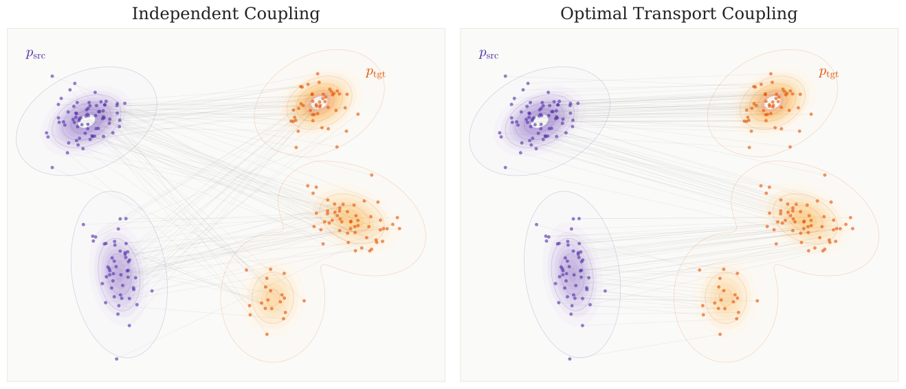
Monge–Kantorovich (Static) Formulation of OT Problem.

We fix a cost function \(c:\mathbb{R}^D\times\mathbb{R}^D\to\mathbb{R}\) that specifies the expense of sending probability mass from \({\mathbf{x}}\) to \({\mathbf{y}}\). The goal is to transform the source distribution \(p_{\mathrm{src}}\) into the target distribution \(p_{\mathrm{tgt}}\) as cheaply as possible.

To even define a cost, we must know which pairs \(({\mathbf{x}},{\mathbf{y}})\) are matched. This role is played by a coupling: a joint distribution \(\gamma\) on \(\mathbb{R}^D\times\mathbb{R}^D\) whose marginals are \(p_{\mathrm{src}}\) and \(p_{\mathrm{tgt}}\). In other words, sampling \(({\mathbf{x}},{\mathbf{y}})\sim\gamma\) means we match \({\mathbf{x}}\) from the source with \({\mathbf{y}}\) from the target. If \(\gamma\) admits a density \(\gamma({\mathbf{x}},{\mathbf{y}})\) with respect to Lebesgue measure, the marginal constraints read \[\int_{\mathbb{R}^D} \gamma({\mathbf{x}},{\mathbf{y}})\,\mathop{}\!\mathrm{d}{\mathbf{y}}= p_{\mathrm{src}}({\mathbf{x}}), \qquad \int_{\mathbb{R}^D} \gamma({\mathbf{x}},{\mathbf{y}})\,\mathop{}\!\mathrm{d}{\mathbf{x}}= p_{\mathrm{tgt}}({\mathbf{y}}).\] That is, integrating out \({\mathbf{y}}\) recovers the source density in \({\mathbf{x}}\), while integrating out \({\mathbf{x}}\) recovers the target density in \({\mathbf{y}}\).

We give two standard examples for illustration:

1. Discrete Supports. If \(p_{\mathrm{src}}\) and \(p_{\mathrm{tgt}}\) are supported on finitely many points, a coupling is represented by a nonnegative matrix \((\gamma_{ij})\) whose row sums equal \(p_{\mathrm{src}}(i)\) and column sums equal \(p_{\mathrm{tgt}}(j)\). Each entry \(\gamma_{ij}\) is the amount of mass sent from \(i\) to \(j\).

2. Deterministic Map. If there exists a measurable map \({\mathbf{T}}\) with \({\mathbf{T}}_\#p_{\mathrm{src}}=p_{\mathrm{tgt}}\), then \(\gamma=({\mathbf{I}},{\mathbf{T}})_\#p_{\mathrm{src}}\) is a deterministic coupling that moves each point \({\mathbf{x}}\) directly to \({\mathbf{T}}({\mathbf{x}})\).

Once a coupling \(\gamma\) is fixed, the transport cost is simply the average unit cost under this plan: \[\int c({\mathbf{x}},{\mathbf{y}})\,\mathop{}\!\mathrm{d}\gamma({\mathbf{x}},{\mathbf{y}}) =\mathbb{E}_{({\mathbf{x}},{\mathbf{y}})\sim\gamma}\!\big[c({\mathbf{x}},{\mathbf{y}})\big].\] In the discrete case, this reduces to \(\sum_{i,j} c_{ij}\gamma_{ij}\), whereas in the continuous setting it becomes a double integral. In what follows, we will focus only on the continuous case.

The optimal transport problem is then to choose, among all admissible couplings, the one that minimizes this expected cost.

where the feasible set simply enforces the marginal, or mass-conservation, constraints: \[\begin{align*} \Gamma(p_{\mathrm{src}},p_{\mathrm{tgt}}) = \Big\{\gamma \in &\mathcal{P}(\mathbb{R}^D\times\mathbb{R}^D): \\ &\int \gamma({\mathbf{x}},{\mathbf{y}}) \mathop{}\!\mathrm{d}{\mathbf{y}}= p_{\mathrm{src}}({\mathbf{x}}),\,\, \int \gamma({\mathbf{x}},{\mathbf{y}})\mathop{}\!\mathrm{d}{\mathbf{x}}= p_{\mathrm{tgt}}({\mathbf{y}})\Big\}, \end{align*}\] where \(\mathcal{P}(\mathbb{R}^D\times\mathbb{R}^D)\) denotes the set of all probability measures on \(\mathbb{R}^D\times\mathbb{R}^D\).

A Special Case: Wasserstein-2 Distance.

The Wasserstein-2 distance is a special case of the Monge–Kantorovich problem with the quadratic cost \(c(\mathbf{x}, \mathbf{y}) = \|\mathbf{x} - \mathbf{y}\|^2\). It measures the distance between two probability distributions as follows: \[\begin{align*} \mathcal{W}_2^2(p_{\mathrm{src}}, p_{\mathrm{tgt}}) := \inf_{\gamma \in \Gamma(p_{\mathrm{src}}, p_{\mathrm{tgt}})} \mathbb{E}_{(\mathbf{x}, \mathbf{y}) \sim \gamma} \left[ \|\mathbf{x} - \mathbf{y}\|^2 \right]. \end{align*}\]

Under suitable assumptions on \(p_{\mathrm{src}}\) and \(p_{\mathrm{tgt}}\), Brenier’s theorem (see Item)¹ guarantees that the optimal coupling \(\gamma\) for the quadratic cost is concentrated on the graph of a deterministic map \({\mathbf{T}}:\mathbb{R}^D \rightarrow \mathbb{R}^D\). Consequently, the Wasserstein-2 distance can be equivalently expressed as²: \[\begin{equation} \label{eq: Monge's Formulation} \mathcal{W}_2^2(p_{\mathrm{src}}, p_{\mathrm{tgt}}) = \inf_{\substack{{\mathbf{T}}:\mathbb{R}^D \rightarrow \mathbb{R}^D,\\ \text{ s.t. }{\mathbf{T}}\#p_{\mathrm{src}} = p_{\mathrm{tgt}}}} \mathbb{E}_{{\mathbf{x}}\sim p_{\mathrm{src}}} \left[ \| {\mathbf{T}}({\mathbf{x}}) - {\mathbf{x}}\|^2 \right]. \end{equation}\] Here, \({\mathbf{T}}\#p_{\mathrm{src}} = p_{\mathrm{tgt}}\) means that \({\mathbf{T}}\) pushes \(p_{\mathrm{src}}\) forward to \(p_{\mathrm{tgt}}\), i.e., \({\mathbf{T}}({\mathbf{x}}) \sim p_{\mathrm{tgt}}\) for \({\mathbf{x}}\sim p_{\mathrm{src}}\).

Thus, the Wasserstein-2 distance represents the minimal expected squared transport cost among all couplings or transport maps that match the given marginals. The optimal transport map denoted by \({\mathbf{T}}^*(\mathbf{x})\), known as the Monge map, yields the most efficient way to transform \(p_{\mathrm{src}}\) into \(p_{\mathrm{tgt}}\).

Benamou–Brenier (Dynamic) Formulation of OT.

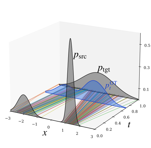
Instead of mapping distributions directly in a static manner, as in the Monge–Kantorovich formulation, transport can also be modeled as a continuous-time flow: \[\begin{equation*} p_0 := p_{\mathrm{src}} \to p_t \to p_1 := p_{\mathrm{tgt}}, \quad t \in [0,1]. \end{equation*}\] This dynamic formulation of optimal transport, introduced by Benamou and Brenier (2000), seeks a smooth velocity field \({\mathbf{v}}_t({\mathbf{x}})\) that describes how mass in \(p_t({\mathbf{x}})\) evolves over time.

The Benamou–Brenier formulation³ shows that, for the quadratic cost \(c({\mathbf{x}}, {\mathbf{y}}) = \|{\mathbf{x}}- {\mathbf{y}}\|_2^2\) (i.e., the \(\mathcal{W}_2\) distance), the optimal value of the static OT problem in Equation \(\eqref{eq:ot}\) is equal to the optimal value of the kinetic energy minimization problem:

where \(p_t\) is a probability distribution on \(\mathbb{R}^D\) for each \(t \in [0,1]\). In particular, The optimal transport flow \(p_t({\mathbf{x}})\) follows McCann’s displacement interpolation: \[\begin{equation*} {\mathbf{T}}_t^*({\mathbf{x}}) = (1 - t){\mathbf{x}}+ t{\mathbf{T}}^*({\mathbf{x}}), \end{equation*}\] where \({\mathbf{T}}^*({\mathbf{x}})\) is the OT map that transports \(p_{\mathrm{src}}\) to \(p_{\mathrm{tgt}}\). This linear interpolation moves mass along straight lines with constant velocity: \(p_t = {\mathbf{T}}_t^*\#p_{\mathrm{src}}\) for each \(t \in [0,1]\).

The optimal transport map \({\mathbf{T}}^*\) satisfies the Monge–Ampère equation:

\[\begin{equation} \label{eq:monge-ampere} p_{\mathrm{tgt}}\left(\nabla \psi({\mathbf{x}})\right) \det\left(\nabla^2 \psi({\mathbf{x}})\right) = p_{\mathrm{src}}({\mathbf{x}}), \end{equation}\] where \({\mathbf{T}}^*({\mathbf{x}}) = \nabla \psi({\mathbf{x}})\) for some convex function \({\bm{\psi}}\) by Brenier’s theorem. However, this nonlinear PDE is typically intractable for explicit solutions. Note that this is precisely the change-of-variables relation used by normalizing flows (c.f., Equation in Chapter 5): flows parametrize an invertible transport map with a tractable Jacobian determinant, but do not in general impose the gradient-of-potential structure \({\mathbf{T}}^*=\nabla\psi\); consequently, a trained flow can differ substantially from the Brenier/OT map.

Entropy-Regularized Optimal Transport (EOT)

To motivate EOT concretely, consider empirical distributions built from samples. Suppose \(p_{\mathrm{src}}\) is supported on points \(\{{\mathbf{x}}^{(i)}\}_{i=1}^n \subset \mathbb{R}^D\) with weights \(a_i\), and \(p_{\mathrm{tgt}}\) on \(\{{\mathbf{y}}^{(j)}\}_{j=1}^n \subset \mathbb{R}^D\) with weights \(b_j\). A coupling is then an \(n\times n\) nonnegative matrix \(\gamma=(\gamma_{ij})\) whose row sums match \(a\) and column sums match \(b\). Each entry \(\gamma_{ij}\) represents the amount of mass transported from \({\mathbf{x}}^{(i)}\) to \({\mathbf{y}}^{(j)}\)⁴.

Why Regularize OT?

Classical OT in this discrete setting (obtained by taking counting measures in the continuous formulation Equation \(\eqref{eq:ot}\)) reduces to minimizing \[\min_{\gamma=(\gamma_{ij})}\sum_{i,j} C_{ij}\,\gamma_{ij},\] over all feasible couplings \(\gamma=(\gamma_{ij})\), where \(C_{ij} = c({\mathbf{x}}^{(i)},{\mathbf{y}}^{(j)})\) is the cost of moving one unit of mass from source point \({\mathbf{x}}^{(i)}\) to target point \({\mathbf{y}}^{(j)}\), for a prescribed ground cost \(c:\mathbb{R}^D\times\mathbb{R}^D\to\mathbb{R}_{\ge 0}\) (e.g., \(c({\mathbf{x}},{\mathbf{y}})=\|{\mathbf{x}}-{\mathbf{y}}\|_2^2\)).

Two main issues arise:

1. Non-Uniqueness and Instability: The minimizer \(\gamma^*\) need not be unique. For example, if two transport plans achieve the same minimum cost, the solver may select either one. Consequently, small changes in the inputs \((a,b,C)\) (such as moving a sample, adjusting weights, or slightly perturbing costs) can cause abrupt jumps in the solution.

2. High Computational Cost: The problem is a linear program with \(n^2\) variables and \(2n\) constraints. Practical solvers (e.g., Hungarian algorithm (Kuhn 1955; Munkres 1957), network simplex (Peyré et al. 2019)) typically scale as \(\mathcal{O}(n^3)\), which is infeasible for large \(n\).

To overcome these bottlenecks, EOT objective function introduces a regularization term to the classical OT problem, controlled by a parameter \(\varepsilon > 0\):

The reference measure \(M\) is typically chosen as the product of the marginals, \(p_{\mathrm{src}} \otimes p_{\mathrm{tgt}}\). The KL divergence term is directly related to the Shannon entropy of the transport plan \(\gamma\): \[\mathcal{D}_{\text{KL}}(\gamma \,\Vert\, p_{\mathrm{src}} \otimes p_{\mathrm{tgt}}) = -\mathcal{H}(\gamma) + \text{Constant},\] where \(\mathcal{H}(\gamma) := -\int \gamma({\mathbf{x}}, {\mathbf{y}}) \log \gamma({\mathbf{x}}, {\mathbf{y}}) \mathop{}\!\mathrm{d}{\mathbf{x}}\mathop{}\!\mathrm{d}{\mathbf{y}}\).

The addition of this regularization term yields several theoretical and practical advantages, which we briefly outline below:

Why Entropy Regularizer Helps?

1. Mass Spreading. Since \(t\mapsto t\log t\) is convex and grows rapidly for large \(t\), minimizing \(\int \gamma\log\gamma\) penalizes peaky couplings (some \(\gamma({\mathbf{x}},{\mathbf{y}})\) very large, most near zero). For fixed total mass \(\int \gamma=1\), it favors plans where \(\gamma({\mathbf{x}},{\mathbf{y}})\) is more evenly distributed over \(({\mathbf{x}},{\mathbf{y}})\in\mathbb{R}^D\times\mathbb{R}^D\). Equivalently, maximizing Shannon entropy promotes higher “uncertainty” (diffuseness).

2. Strict Convexity and Uniqueness. Because \(\mathcal{H}\) is strictly concave, the objective in Equation \(\eqref{eq:eot-epsilon}\) is strictly convex in \(\gamma\), yielding a unique minimizer \(\gamma^*_\varepsilon\) that depends continuously on \((p_{\mathrm{src}},p_{\mathrm{tgt}},c)\).

3. Sinkhorn Form and Positivity. Under mild conditions⁵, the optimizer has the Schrödinger/Sinkhorn form \[\gamma^*_\varepsilon({\mathbf{x}},{\mathbf{y}}) = u({\mathbf{x}})\, \exp \bigl(-\tfrac{c({\mathbf{x}},{\mathbf{y}})}{\varepsilon}\bigr) \,v({\mathbf{y}})p_{\mathrm{src}}({\mathbf{x}}) p_{\mathrm{tgt}}({\mathbf{y}}),\] for positive scaling functions \(u,v\) (unique up to a global factor). In practice, the continuous formulation is approximated with finite samples, reducing EOT to a finite (sampled) Sinkhorn iteration. The entropic objective is strictly convex, and the scaling (Sinkhorn/IPFP) algorithm solves it efficiently (Sinkhorn 1964; Cuturi 2013). For a dense problem with \(n\) support points per marginal (an \(n\times n\) kernel), each Sinkhorn iteration costs \(\mathcal{O}(n^2)\) time and \(\mathcal{O}(n^2)\) memory, making the method more scalable and practical (Altschuler et al. 2017).

4. Limits in \(\varepsilon\). As \(\varepsilon \to 0\), the optimal plan \(\gamma^*_\varepsilon\) becomes increasingly concentrated, approaching a (possibly singular) classical OT coupling (we will revisit this connection in Section 1.3.2). As \(\varepsilon\) increases, \(\gamma^*_\varepsilon\) gradually spreads out and approaches the independent coupling \(p_{\mathrm{src}}\otimes p_{\mathrm{tgt}}\).

Schrödinger Bridge (SB)

KL Formulation of SB.

The Schrödinger Bridge (SB) problem, introduced by Erwin Schrödinger in the 1930s, asks the following question. Suppose particles move according to some simple reference dynamics, such as Brownian motion. Now imagine that we observe the particles at two times: at \(t=0\) their distribution is \(p_{\mathrm{src}}\), and at \(t=1\) it is \(p_{\mathrm{tgt}}\). Among all possible stochastic processes that connect these two distributions, which one deviates the least from the reference dynamics? Here “deviation” is measured by the KL divergence, so the solution to the SB problem is the most likely way to deform Brownian motion into a process that satisfies the prescribed boundary conditions.

To make this precise, let \({\mathbf{x}}_{0:T}:=\{{\mathbf{x}}_t\}_{t\in[0,T]}\) denote a complete trajectory of the process. We write \(P\) for the law of trajectories, that is, the probability distribution over entire sample paths. The time-\(t\) marginal of \(P\) is denoted by \(p_t\) (or \(P_t\)), which describes the distribution of the state \({\mathbf{x}}_t\) at a single time. Formally, for a measurable set \(A\subseteq\mathbb R^D\), \[p_t(A) = P({\mathbf{x}}_t \in A).\] In other words, \(p_t\) can be viewed as the empirical distribution obtained by sampling many full trajectories from \(P\) and then collecting the states at time \(t\)—for instance, as a histogram if the state is one-dimensional.

Consider a reference diffusion \(\{{\mathbf{x}}_t\}_{t\in[0,T]}\) governed by the SDE \[\begin{align} \label{eq:general-sb-sde} \mathop{}\!\mathrm{d}{\mathbf{x}}_t = {\mathbf{f}}({\mathbf{x}}_t,t)\,\mathop{}\!\mathrm{d}t + g(t)\,\mathop{}\!\mathrm{d}{\mathbf{w}}_t, \end{align}\] where \({\mathbf{f}}\colon \mathbb{R}^D\times[0,T]\!\to\!\mathbb{R}^D\), \(g\colon[0,T]\!\to\!\mathbb{R}\), and \(\{{\mathbf{w}}_t\}_{t\in[0,T]}\) is a standard Brownian motion. Let \(R\) denote the path law (joint distribution) of the full trajectory \({\mathbf{x}}_{0:T}:=\{{\mathbf{x}}_t\}_{t\in[0,T]}\), and let \(R_0\) denote the initial marginal of the reference process; this \(R\) will serve as the reference trajectory distribution.

With this notation, the SB problem seeks a trajectory law \(P\) that is closest to \(R\) in KL divergence while matching the prescribed endpoint marginals: \[\begin{align} \label{eq:sb-epsilon-general} \mathrm{SB}(p_{\mathrm{src}}, p_{\mathrm{tgt}}) := \min_{P}\, \mathcal{D}_{\mathrm{KL}}(P\|R) \quad \text{s.t.} \quad P_0 = p_{\mathrm{src}},\;\; P_T = p_{\mathrm{tgt}}. \end{align}\] The optimizer \(P^*\) depends on the chosen reference process \(R\).

Stochastic Control View of SB.

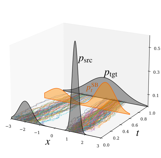
Rather than optimizing over arbitrary path distributions \(P\) in Equation \(\eqref{eq:sb-epsilon-general}\), a more tractable approach is to take the reference dynamics as an anchor and allow it to drift. This is done by introducing a time-dependent drift \({\mathbf{v}}_t({\mathbf{x}}_t)\), which perturbs the reference process and generates a family of candidate trajectory distributions. The resulting dynamics take the form of a controlled diffusion: \[\mathop{}\!\mathrm{d}{\mathbf{x}}_t = \bigl[{\mathbf{f}}({\mathbf{x}}_t,t) + {\mathbf{v}}_t({\mathbf{x}}_t)\bigr]\mathop{}\!\mathrm{d}t + g(t) \mathop{}\!\mathrm{d}{\mathbf{w}}_t,\] where \({\mathbf{v}}_t:\mathbb{R}^D\to\mathbb{R}^D\) is the drift to be optimized later (Equation \(\eqref{eq:sb-kinetic}\)). Under standard integrability conditions (e.g., Novikov’s condition) and by Girsanov’s theorem (see Section (Girsanov’s Theorem as a Bridge Between Likelihood Training and Score Matching) in Appendix C), the KL divergence between the controlled law \(P\) and the reference \(R\) admits the dynamic (kinetic) form \[\begin{align*} \mathcal{D}_{\mathrm{KL}}(P\|R) &= \mathcal{D}_{\mathrm{KL}}(p_{\mathrm{src}}\|R_0) + \mathbb{E}_{P}\!\left[ \frac{1}{2}\int_0^T \frac{\|{\mathbf{v}}_t({\mathbf{x}}_t)\|^2}{g^2(t)} \mathop{}\!\mathrm{d}t \right] \\ &= \mathcal{D}_{\mathrm{KL}}(p_{\mathrm{src}}\|R_0) + \frac{1}{2}\int_0^T\!\int_{\mathbb{R}^D} \frac{\|{\mathbf{v}}_t({\mathbf{x}})\|^2}{g^2(t)} p_t({\mathbf{x}})\mathop{}\!\mathrm{d}{\mathbf{x}}\mathop{}\!\mathrm{d}t . \end{align*}\] where \(p_t\) is the time–\(t\) marginal of \({\mathbf{x}}_t\) under the controlled process. The second equality follows from the law of total expectation. Since \(P_0=p_{\mathrm{src}}\) is fixed in the SB problem, the first term is constant with respect to the control and may therefore be omitted from the optimization. In particular, it vanishes when \(R_0=p_{\mathrm{src}}\).

Hence, the SB problem can be reformulated as minimizing the expected control energy over all admissible drifts \({\mathbf{v}}_t\) that steer the process from \(p_{\mathrm{src}}\) at \(t=0\) to \(p_{\mathrm{tgt}}\) at \(t=T\) (Dai Pra 1991; Pra and Pavon 1990; Pavon and Wakolbinger 1991; Chen et al. 2016). Since the initial marginal is fixed to \(p_{\mathrm{src}}\), we may take the reference process to have \(R_0=p_{\mathrm{src}}\) without changing the optimizer; then \(\mathcal{D}_{\mathrm{KL}}(p_{\mathrm{src}}\|R_0)=0\). This leads to the stochastic control formulation:

Importantly, the endpoint distributions \(p_{\mathrm{src}}\) and \(p_{\mathrm{tgt}}\) are arbitrary; the control \({\mathbf{v}}_t\) is chosen precisely to “bridge” the reference dynamics between these marginals while staying as close as possible (in KL divergence) to the reference process \(R\).

A Special Brownian Reference.

Equation \(\eqref{eq:sb-kinetic}\) resembles the Benamou–Brenier formulation of OT in Equation \(\eqref{eq:bb-ot}\), especially when the reference process \(R^\varepsilon\) (with \(\varepsilon>0\)) is chosen to be a Brownian motion⁶: \[\mathop{}\!\mathrm{d}{\mathbf{x}}_t = \sqrt{\varepsilon}\,\mathop{}\!\mathrm{d}{\mathbf{w}}_t,\] so that \({\mathbf{f}}\equiv \mathbf{0}\) and \(g(t) \equiv \sqrt{\varepsilon}\).

In this setting, the SB problem seeks a path distribution \(P\) that stays closest (in KL divergence) to the Brownian reference \(R^\varepsilon\), while matching the endpoint marginals: \[\begin{align} \label{eq:sb-epsilon} \mathrm{SB}_\varepsilon(p_{\mathrm{src}}, p_{\mathrm{tgt}}) := \min_{P} \mathcal{D}_{\mathrm{KL}}(P \| R^\varepsilon) \quad \text{s.t.} \quad P_0 = p_{\mathrm{src}}, \;\; P_T = p_{\mathrm{tgt}}. \end{align}\] The equivalent stochastic control formulation then becomes \[\begin{align} \label{eq:sb-epsilon-kinetic} \begin{aligned} \mathrm{SB}_\varepsilon(p_{\mathrm{src}}, p_{\mathrm{tgt}}) = \min_{\substack{ {\mathbf{v}}_t \text{ s.t. } \mathop{}\!\mathrm{d}{\mathbf{x}}_t = {\mathbf{v}}_t({\mathbf{x}}_t)\,\mathop{}\!\mathrm{d}t + \sqrt{\varepsilon}\,\mathop{}\!\mathrm{d}{\mathbf{w}}_t, \\ {\mathbf{x}}_0 \sim p_{\mathrm{src}},\;\; {\mathbf{x}}_T \sim p_{\mathrm{tgt}} }} \frac{1}{2\varepsilon}\int_0^T \!\!\int_{\mathbb{R}^D} \|{\mathbf{v}}_t({\mathbf{x}})\|^2 \, p_t({\mathbf{x}})\,\mathop{}\!\mathrm{d}{\mathbf{x}}\,\mathop{}\!\mathrm{d}t, \end{aligned} \end{align}\] where \(p_t\) denotes the time–\(t\) marginal of diffusion driven by the drift \({\mathbf{v}}_t\): \[\mathop{}\!\mathrm{d}{\mathbf{x}}_t = {\mathbf{v}}_t({\mathbf{x}}_t)\,\mathop{}\!\mathrm{d}t + \sqrt{\varepsilon}\,\mathop{}\!\mathrm{d}{\mathbf{w}}_t.\]

Why We Need to Specify a Reference Distribution?

Classical OT does not require a reference path distribution because the prescribed ground cost already tells us how expensive it is to pair a source point with a target point. The optimization therefore compares admissible couplings directly through this cost. In the SB problem, however, we compare entire stochastic trajectories rather than only their endpoints. We therefore need a reference path measure \(R\) that specifies what the uncontrolled dynamics would normally look like. The quantity \(\mathcal{D}_{\mathrm{KL}}(P\|R)\) then measures how much an admissible process \(P\) must deviate from these reference dynamics in order to satisfy the prescribed endpoint distributions.

Coupled PDE Characterization.

A convenient way to describe the SB solution is through two space–time potentials \(\Psi(x,t)\) and \(\widehat{\Psi}(x,t)\). Let \(p_t^{\mathrm{SB}}\) denote the marginal at time \(t\in[0,T]\) of the optimal trajectory law \(P^*\) in Equation \(\eqref{eq:sb-epsilon-general}\). Then one has the symmetric factorization (Dai Pra 1991) \[\begin{align} \label{eq:sb-symmetry} p_t^{\mathrm{SB}}(x) = \Psi(x,t) \widehat{\Psi}(x,t), \end{align}\] where \(\Psi\) and \(\widehat{\Psi}\) solve the (linear) Schrödinger system (Caluya and Halder 2021; Chen et al. 2021; Chen et al. 2022): \[\begin{align} \begin{aligned}\label{eq:pde-schrodinger} \frac{\partial \Psi}{\partial t}(\mathbf{x},t) &= -\nabla_{\mathbf{x}} \Psi(\mathbf{x},t) \cdot {\mathbf{f}}(\mathbf{x},t) - \frac{g^2(t)}{2}\,\Delta_\mathbf{x} \Psi(\mathbf{x},t), \\ \frac{\partial \widehat{\Psi}}{\partial t}(\mathbf{x},t) &= -\nabla_{\mathbf{x}}\!\cdot\!\bigl(\widehat{\Psi}(\mathbf{x},t)\,{\mathbf{f}}(\mathbf{x},t)\bigr) + \frac{g^2(t)}{2}\,\Delta_\mathbf{x}\widehat{\Psi}(\mathbf{x},t) \\ \text{subject to}\quad \Psi(\mathbf{x},0)&\,\widehat{\Psi}(\mathbf{x},0) = p_{\mathrm{src}}(\mathbf{x}), \quad \Psi(\mathbf{x},T)\,\widehat{\Psi}(\mathbf{x},T) = p_{\mathrm{tgt}}(\mathbf{x}). \end{aligned} \end{align}\]

Forward-Time Schrödinger Bridge SDE.

Once \(\Psi\) is known, the optimal dynamics is the reference diffusion tilted by the space–time factor \(\Psi\): \[\begin{align} \label{eq:sb-forward-sde} \mathop{}\!\mathrm{d}{\mathbf{x}}_t = \bigl[{\mathbf{f}}({\mathbf{x}}_t, t) + g^2(t)\,\nabla_{\mathbf{x}} \log \Psi({\mathbf{x}}_t, t)\bigr]\mathop{}\!\mathrm{d}t + g(t)\mathop{}\!\mathrm{d}{\mathbf{w}}_t, \quad {\mathbf{x}}_0 \sim p_{\mathrm{src}}. \end{align}\] Let \(Q\) denote the trajectory law of Equation \(\eqref{eq:sb-forward-sde}\) (so \(Q_0=p_{\mathrm{src}}\) and \(Q_T=p_{\mathrm{tgt}}\) by Equation and Equation). Then \(Q=P^*\) and the minimizer \({\mathbf{v}}^*\) to Equation \(\eqref{eq:sb-kinetic}\) is (see (Chen et al. 2021)’s Section 4.6): \[{\mathbf{v}}_t^{*}({\mathbf{x}}) = g^2(t) \nabla_{\mathbf{x}}\log \Psi({\mathbf{x}},t).\] That is, drift correction \(g^2\nabla_{\mathbf{x}}\log\Psi\) is precisely the minimal KL perturbation of the reference needed to match the endpoint marginals.

Reverse-Time Schrödinger Bridge SDE.

The same optimal path law can be generated reverse in time. A convenient way to see the form of the reverse-time drift is to conceptually use the standard time-reversal identity for diffusions: \[{\mathbf{b}}^{-}({\mathbf{x}},t)={\mathbf{b}}^{+}({\mathbf{x}},t)-g^2(t)\nabla_{\mathbf{x}}\log p_t^{\mathrm{SB}}({\mathbf{x}}),\] where \({\mathbf{b}}^{+}={\mathbf{f}}+g^2\nabla\log\Psi\) and \(p_t=\Psi\,\widehat{\Psi}\). This gives \[{\mathbf{b}}^{-}({\mathbf{x}},t)={\mathbf{f}}({\mathbf{x}},t)-g^2(t) \nabla_{\mathbf{x}}\log \widehat{\Psi}({\mathbf{x}},t).\] Thus the reverse-time SDE reads \[\begin{align} \label{eq:sb-backward-sde} \mathop{}\!\mathrm{d}{\mathbf{x}}_t = \Big[{\mathbf{f}}({\mathbf{x}}_t,t) - g^2(t) \nabla_{{\mathbf{x}}}\log \widehat{\Psi}({\mathbf{x}}_t,t)\Big]\mathop{}\!\mathrm{d}t + g(t)\,\mathop{}\!\mathrm{d}\bar{{\mathbf{w}}}_t, \quad {\mathbf{x}}_T \sim p_{\mathrm{tgt}} . \end{align}\] Equivalently, reparametrizing time by \({\mathbf{y}}_\tau := {\mathbf{x}}_{T-\tau}\) so that \(\tau\) increases from \(0\) to \(T\). Then \({\mathbf{y}}_\tau\) evolves forward in \(\tau\) from \({\mathbf{y}}_0 \sim p_{\mathrm{tgt}}\) as \[\begin{align} \label{eq:sb-reverse-forward-tau} \begin{aligned} \mathop{}\!\mathrm{d}{\mathbf{y}}_\tau = \big[-{\mathbf{f}}({\mathbf{y}}_\tau,T-\tau) + g^2(T-\tau) \nabla_{{\mathbf{y}}}\log \widehat{\Psi}({\mathbf{y}}_\tau,T-\tau)\big]\mathop{}\!\mathrm{d}\tau + g(T-\tau) \mathop{}\!\mathrm{d}{\mathbf{w}}_\tau. \end{aligned} \end{align}\]

Both the forward and reverse descriptions yield the same optimal path law \(P^*\) which are linked by \[\nabla\log p_t^{\mathrm{SB}}=\nabla\log\Psi+\nabla\log\widehat\Psi, \qquad {\mathbf{b}}^{-}={\mathbf{b}}^{+}-g^2\,\nabla\log p_t^{\mathrm{SB}},\] so their marginals coincide with \(p_t^{\mathrm{SB}}\) at every time. The additional drift terms \(g^2\nabla\log\Psi\) (forward) and \(-\,g^2\nabla\log\widehat{\Psi}\) (reverse-time) act as control forces that steer the reference diffusion to match the endpoint marginals while staying closest to the reference in relative entropy.

Practical Obstacles to the Coupled PDE Approach.

To construct the generative process based on Equation \(\eqref{eq:sb-backward-sde}\), one must solve the coupled PDEs in Equation \(\eqref{eq:pde-schrodinger}\) to obtain the backward Schrödinger potential \(\widehat{\Psi}\). However, these PDEs are notoriously difficult to solve, even in low-dimensional settings, which makes their direct application in generative modeling challenging. To circumvent this, several works have proposed alternative strategies: leveraging Score SDE techniques to iteratively solve each half-bridge problem (\(p_{\mathrm{tgt}} \leftarrow p_{\mathrm{src}}\) and \(p_{\mathrm{tgt}} \rightarrow p_{\mathrm{src}}\)) (De Bortoli et al. 2021); optimizing surrogate likelihood bounds (Chen et al. 2022; Liu et al. 2023); or designing simulation-free training based on an analytical solution of the posterior \({\mathbf{x}}_t \vert {\mathbf{x}}_0, {\mathbf{x}}_T\) for sample pairs \(({\mathbf{x}}_0, {\mathbf{x}}_T) \sim p_{\mathrm{src}} \otimes p_{\mathrm{tgt}}\) (Liu et al. 2023). We do not delve into the technical details here but briefly discuss the connection between diffusion models and SB in Section 1.4.

Global Pushforwards and Local Dynamics: An OT Analogy for DGMs

From the optimal-transport viewpoint (in Equation \(\eqref{eq:ot}\)), one can leverage deep generative models to learn a transport (pushforward) map from a simple prior to the data, i.e., \({\mathbf{G}}_{\bm{\phi}\#}p_{\mathrm{prior}} \approx p_{\mathrm{data}}\). Although \({\mathbf{G}}_{\bm{\phi}}\) generally does not coincide with the optimal transport map (except in works (Genevay et al. 2018; Onken et al. 2021) that impose an OT objective under suitable conditions), the Benamou–Brenier formulation (in Equation \(\eqref{eq:bb-ot}\)) provides a complementary, dynamic perspective. Rather than directly learning a single global map, it describes transport as a continuous flow generated by a time-dependent local vector field, tracing a smooth path between \(p_{\mathrm{prior}}\) and \(p_{\mathrm{data}}\). This dynamic formulation parallels the relationship between the static Schrödinger Bridge problem (in Equation \(\eqref{eq:sb-epsilon-general}\)) and its stochastic-control counterpart (in Equation \(\eqref{eq:sb-kinetic}\)), where the optimal coupling is realized as a controlled diffusion process. A similar analogy emerges in generative modeling: standard DGMs such as GANs or VAEs learn a global pushforward map, whereas diffusion models learn a time-dependent local vector field that drives the generative dynamics.

Relationship of Variant Optimal Transport Formulations

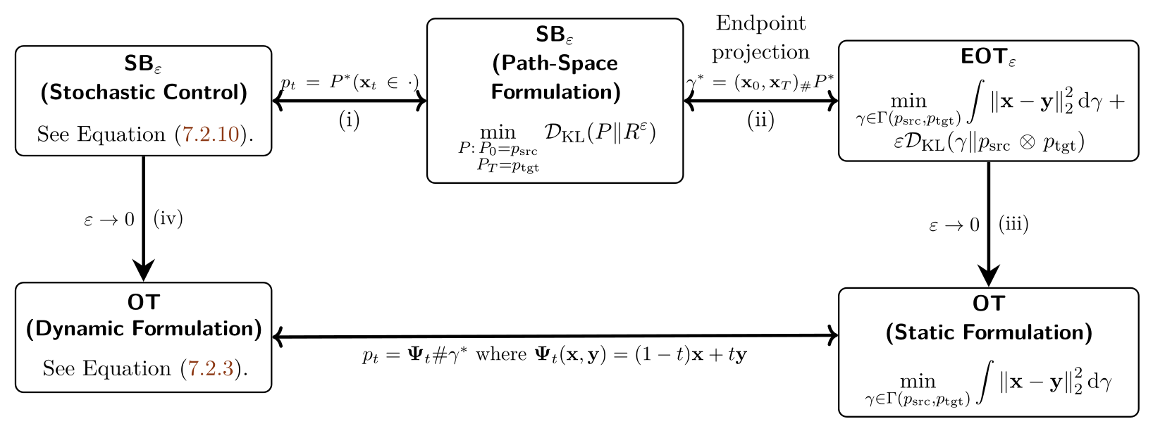
Before delving into the technical details, it is helpful to clarify how the different formulations of optimal transport and its entropic regularizations are connected. At a high level, these problems can be viewed as related (see Figure 1.4 for their diagram for connection):

1. Path-Space SB \(\Longleftrightarrow\) Stochastic-Control SB. The path-space KL formulation of \(\mathrm{SB}_\varepsilon\) and its stochastic-control formulation describe the same bridge problem relative to the chosen reference process (see Section 1.2.3).

2. Brownian-Reference SB \(\Longleftrightarrow\) EOT\(_\varepsilon\). For the Brownian reference \[\mathop{}\!\mathrm{d}{\mathbf{x}}_t=\sqrt{\varepsilon}\,\mathop{}\!\mathrm{d}{\mathbf{w}}_t,\] with the corresponding quadratic-cost normalization, the endpoint coupling induced by the optimal SB path law solves the associated \(\mathrm{EOT}_\varepsilon\) problem (see Section 1.3.1).

3. EOT\(_\varepsilon\) \(\longrightarrow\) Static OT. As \(\varepsilon\to0\), the entropy-regularized endpoint coupling approaches the corresponding classical OT problem, and the optimal values converge to the OT value under the assumptions discussed in Section 1.3.2.

4. SB\(_\varepsilon\) \(\longrightarrow\) Dynamic OT. Under the corresponding small-noise scaling, the Brownian-reference Schrödinger problem converges as \(\varepsilon\to0\) to the Benamou–Brenier dynamic formulation of OT (see Section 1.3.3).

Together, these non-trivial relationships provide a compact view across stochastic control, entropy-regularized, and classical OT frameworks.

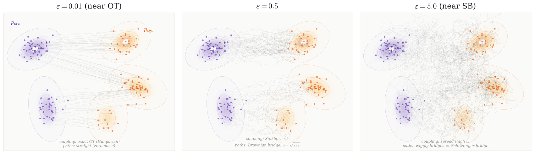
SB and EOT are (Dual) Equivalent

In this section, we present two complementary perspectives showing that SB are essentially equivalent to EOT. Unlike classical optimal transport, which produces a single deterministic map, SB yields a stochastic flow of particles: mass is transported probabilistically, with marginals evolving under diffusion-like dynamics.

From the static viewpoint, SB coincides with EOT, where the goal is to find a coupling between the two endpoint distributions that balances transport cost with entropy. From the dynamic viewpoint, SB describes a controlled diffusion process that remains as close as possible to a simple reference (such as Brownian motion) while still matching the desired endpoints. Each perspective independently establishes the equivalence, providing two consistent ways to understand SB/EOT as canonical formulations of distribution-to-distribution transformation.

Static Schrödinger Bridge.

Let \[\widetilde R^\varepsilon({\mathbf{x}},{\mathbf{y}}) := \frac{1}{Z_\varepsilon}\,e^{-c({\mathbf{x}},{\mathbf{y}})/\varepsilon}\,p_{\mathrm{src}}({\mathbf{x}})\,p_{\mathrm{tgt}}({\mathbf{y}}),\] with normalizing constant \[Z_\varepsilon := \iint e^{-c({\mathbf{x}}, {\mathbf{y}})/\varepsilon}\, p_{\mathrm{src}}({\mathbf{x}})\, p_{\mathrm{tgt}}({\mathbf{y}})\,\mathrm d{\mathbf{x}}\,\mathrm d{\mathbf{y}}.\] Then, for any admissible coupling \(\gamma\in\Gamma(p_{\mathrm{src}},p_{\mathrm{tgt}})\), a direct computation gives \[\int c\, \mathrm d\gamma +\varepsilon \mathcal{D}_\mathrm{KL}\!\bigl(\gamma \Vert p_{\mathrm{src}}\!\otimes\!p_{\mathrm{tgt}}\bigr) = \varepsilon \mathcal{D}_\mathrm{KL}\!\bigl(\gamma \Vert \widetilde R^\varepsilon\bigr) -\varepsilon\log Z_\varepsilon.\] Therefore, \[\begin{align} \begin{aligned}\label{eq:eot-sb-static} \min_{\gamma\in\Gamma(p_{\mathrm{src}},p_{\mathrm{tgt}})} \Bigl\{\int c \,\mathrm d\gamma + \varepsilon \mathcal{D}_\mathrm{KL}\!\bigl(\gamma \Vert p_{\mathrm{src}}\!\otimes\!p_{\mathrm{tgt}}\bigr)\Bigr\} = \varepsilon \min_{\gamma\in\Gamma(p_{\mathrm{src}},p_{\mathrm{tgt}})} &\mathcal{D}_\mathrm{KL}\!\bigl(\gamma \Vert \widetilde R^\varepsilon\bigr) \\&-\varepsilon\log Z_\varepsilon, \end{aligned} \end{align}\] so the entropic OT problem is equivalent, up to an additive constant, to the static Schrödinger Bridge problem \[\min_{\gamma\in\Gamma(p_{\mathrm{src}},p_{\mathrm{tgt}})} \mathcal{D}_\mathrm{KL}(\gamma\Vert \widetilde R^\varepsilon).\]

Dynamic Equivalence (Brownian Reference).

We can also understand this equivalence from a dynamical viewpoint. A classical result (Mikami and Thieullen 2006) states that entropic OT with quadratic cost \[c({\mathbf{x}},{\mathbf{y}})=\frac{\|{\mathbf{y}}-{\mathbf{x}}\|^2}{2T}\] is affinely equivalent to the SB problem where the reference path law \(R^\varepsilon\) is Brownian motion on \([0,T]\), \[\mathrm{d}{\mathbf{x}}_t=\sqrt{\varepsilon}\,\mathrm{d}{\mathbf{w}}_t.\] Here, “affinely equivalent” means the optimal values differ by a positive scaling and an additive constant (independent of the decision variable), so the minimizers coincide. In particular, let \(P^*\) be the optimal path distribution for SB. The key connection to EOT is obtained by looking only at the two endpoints of this optimal stochastic process. If \({\mathbf{x}}_{[0:T]}\sim P^*\), then the endpoint pair \(({\mathbf{x}}_0,{\mathbf{x}}_T)\) induces the coupling \[\gamma^*:=({\mathbf{x}}_0,{\mathbf{x}}_T)_\#P^*,\] and \(\gamma^*\) is an optimal transport plan for the corresponding EOT problem.

Conversely, starting from an optimal EOT coupling \(\gamma^*\), we may first sample a pair of endpoints \(({\mathbf{x}}_0,{\mathbf{x}}_T)\sim\gamma^*\) and then, conditioned on these endpoints, sample a trajectory from the reference diffusion conditioned to connect \({\mathbf{x}}_0\) to \({\mathbf{x}}_T\). Mixing these conditional diffusion paths according to \(\gamma^*\) recovers the optimal SB path distribution \(P^*\).

In words, the optimal stochastic process from the dynamic SB problem induces the optimal endpoint coupling of the static EOT problem. Conversely, the optimal EOT coupling specifies how the endpoints should be paired, while the reference diffusion specifies the optimal stochastic path between each paired set of endpoints.

The key idea to derive this fact is that the KL divergence over paths can be broken down according to the endpoints, which means the Schrödinger bridge problem reduces to a KL divergence just over the joint distribution of \(({\mathbf{x}}_0,{\mathbf{x}}_T)\). For Brownian motion the transition density between \({\mathbf{x}}\) and \({\mathbf{y}}\) has a Gaussian form, so its negative log is quadratic: \[-\varepsilon\log p_T({\mathbf{y}}\mid{\mathbf{x}})=\frac{\|{\mathbf{y}}-{\mathbf{x}}\|^2}{2T}+\text{const}.\] This shows that the endpoint KL is exactly the same as the entropic OT objective with quadratic cost, up to an irrelevant constant.

SB with General Reference Determines the Endpoint EOT Cost.

The connection between SB and EOT is not restricted to Brownian motion. For a general well-posed reference process, its transition law tells us how “natural” it is under the reference dynamics to move from \({\mathbf{x}}\) at time \(0\) to \({\mathbf{y}}\) at time \(T\). Endpoint pairs that are unlikely under the reference should therefore carry a larger transport cost.

More precisely, let \(p_T({\mathbf{y}}|{\mathbf{x}})\) denote the transition density of the reference process over \([0,T]\). Up to a scaling and additive terms that depend only on the fixed endpoint marginals, the corresponding endpoint cost takes the form \[c({\mathbf{x}},{\mathbf{y}}) \propto -\log p_T({\mathbf{y}}|{\mathbf{x}}).\] Thus, at the level of endpoint couplings, the reference dynamics induce the cost used by the corresponding EOT problem: likely transitions receive smaller cost, while unlikely transitions receive larger cost.

The full reference process contains additional information beyond this endpoint cost. Once an endpoint pair \(({\mathbf{x}},{\mathbf{y}})\) is selected, the reference dynamics also determine the conditional stochastic paths used to connect those endpoints. In this sense, EOT determines how the endpoints are optimally paired, while SB additionally describes the stochastic transport between each paired set of endpoints.

EOT\(_\varepsilon\) is Reduced to OT as \(\varepsilon\to 0\)

Let \(\gamma^*_\varepsilon\) denote the optimal plan for \(\mathrm{EOT}_\varepsilon\), and let \(\gamma^*\) denote an optimal plan of the unregularized OT problem in Equation \(\eqref{eq:ot}\). Under standard assumptions, as \(\varepsilon\to0\) the EOT optimal values converge to the OT value, and any limiting entropic optimal plan is OT-optimal; when the OT optimizer is unique, the optimal plans converge to \(\gamma^*\).

This convergence result is both fundamental and practically important. One of the reasons is that the entropy-regularized OT problem \(\mathrm{EOT}_\varepsilon\) admits efficient numerical solutions via algorithms such as Sinkhorn. Thus, the result provides theoretical justification for using \(\mathrm{EOT}_\varepsilon\) with small \(\varepsilon\) as a computationally tractable proxy for the classical OT problem in Equation \(\eqref{eq:ot}\), even when the cost function \(c({\mathbf{x}}, {\mathbf{y}})\) is more general than the quadratic case.

SB\(_\varepsilon\) is Reduced to OT as \(\varepsilon\to 0\)

For direct comparison with Equation \(\eqref{eq:bb-ot}\), we rescale time so that \(T=1\) throughout this subsection. For each \(\varepsilon > 0\), let \(\mathbf{v}_t^\varepsilon\) be a minimizer of the SB problem as in Equation \(\eqref{eq:sb-epsilon-kinetic}\), and let \(p_t^\varepsilon\) be the marginal distribution of the controlled SDE \(\mathbf{x}_t\) induced by \(\mathbf{v}_t^\varepsilon\). Then \(p_t^\varepsilon\) satisfies the associated Fokker–Planck equation. In contrast, denote by \((p_t^0, \mathbf{v}_t^0)\) a minimizer of the Benamou–Brenier formulation of optimal transport (see Equation \(\eqref{eq:bb-ot}\)).

The following theorem⁷ states that as \(\varepsilon \to 0\), the SB problem converges to the OT problem. This result is practically important for reasons similar to those in Theorem: (Informal) EOT_ε Converges to OT. The objective \(\mathrm{SB}_\varepsilon\) can be efficiently solved using Sinkhorn type algorithms, yielding a numerically tractable and differentiable proxy for optimal transport. This is especially valuable in high dimensional or large scale settings, where direct solvers (e.g., based on the Benamou–Brenier formulation) become computationally expensive.

Until now, we have presented the fundamental equivalences (under their respective assumptions) between EOT and SB, as well as their important connection to OT through a limiting process, illustrated in Figure 1.4. Next, we will explore how diffusion models connect to these concepts.

Is Diffusion Model’s SDE Optimal Solution to SB Problem?

Diffusion models as a Special Case of Schrödinger Bridges

SB framework extends (score-based) diffusion models by enabling nonlinear interpolation between arbitrary source and target distributions. It achieves this by adding control drift terms derived from scalar potentials \(\Psi(\mathbf{x}, t)\) and \(\widehat{\Psi}(\mathbf{x}, t)\), which guide a reference diffusion process to match prescribed endpoint marginals (see Equation \(\eqref{eq:pde-schrodinger}\)) and follow the decomposition: \[\nabla\log{\Psi(x,t)}+\nabla\log{\hat{\Psi}(x,t)}=\nabla \log p_t^{\mathrm{SB}}(\mathbf{x}).\] This generalization allows the model to move beyond standard Gaussian priors and generate samples from broader distributions.

Connection to Diffusion Models.

Diffusion models arise as a special case of the SB framework. Suppose the potential is constant, \(\Psi(\mathbf{x}, t) \equiv 1\). Under this assumption, the second PDE in Equation \(\eqref{eq:pde-schrodinger}\) reduces to the standard Fokker–Planck equation, whose solution is the marginal density of the reference process: \[\begin{align} \label{eq:sb-backward-potential} \widehat{\Psi}(\mathbf{x}, t) = p_t^{\mathrm{SB}}(\mathbf{x}). \end{align}\] The corresponding SB forward SDE thus becomes the uncontrolled reference process: \[\mathop{}\!\mathrm{d}\mathbf{x}_t = \mathbf{f}(\mathbf{x}_t, t)\mathop{}\!\mathrm{d}t + g(t)\mathop{}\!\mathrm{d}\mathbf{w}_t,\] and the SB backward SDE simplifies to: \[\mathop{}\!\mathrm{d}\mathbf{x}_t = \left[\mathbf{f}(\mathbf{x}_t, t) - g^2(t) \nabla \log p_t^{\mathrm{SB}}(\mathbf{x}_t) \right]\mathop{}\!\mathrm{d}t + g(t)\mathop{}\!\mathrm{d}\bar{\mathbf{w}}_t,\] which matches Anderson’s reverse-time SDE used in diffusion models. This correspondence shows that diffusion models can be interpreted as the zero-control limit of SB, where no additional drift is introduced by the potentials.

Boundary Conditions and Generality.

The above reduction is purely formal unless the boundary constraints are compatible. For arbitrary source/target \((p_{\mathrm{src}},p_{\mathrm{tgt}})\), the PDE boundary conditions in Equation \(\eqref{eq:pde-schrodinger}\) are generally not satisfied by the choice \(\Psi\equiv 1\). Full SB resolves this by learning nontrivial potentials that induce a nonlinear control drift, bending the reference dynamics to match any prescribed endpoints. By contrast, diffusion models fix one endpoint to a simple prior (typically Gaussian) and learn only the reverse-time score to reach the data. With this perspective, SB is the more flexible umbrella: with nontrivial potentials it bridges arbitrary endpoints; with \(\Psi\equiv 1\) it collapses to the diffusion-model case above. We additionally remark that in the standard linear diffusion model, \(p_T \approx p_{\mathrm{prior}}\) holds only as \(T \to \infty\), so the match to the prior is merely approximate.

Diffusion Models as Schrödinger Half-Bridges

In this section, we explain why diffusion models are not full Schrödinger bridges, but can instead be understood through the relaxed notion of Schrödinger half-bridges. A half-bridge enforces only one endpoint constraint (either \(p_{\mathrm{prior}}\) or \(p_{\mathrm{data}}\)) rather than both, making it a one-sided variant of the full bridge. Before formalizing this connection, we introduce the definition of Schrödinger half-bridges, building on the general formulation in Equation \(\eqref{eq:sb-epsilon-general}\) with arbitrary \(p_{\mathrm{src}}\) and \(p_{\mathrm{tgt}}\). We will then return to diffusion models and show how the half-bridge viewpoint naturally applies when the endpoints are given by \(p_{\mathrm{prior}}\) and \(p_{\mathrm{data}}\).

Schrödinger Half-Bridges

The SB problem asks for a stochastic process whose law is closest (in KL divergence) to a simple reference process, while matching two endpoint distributions \(p_{\mathrm{src}}\) and \(p_{\mathrm{tgt}}\). Solving the full bridge requires enforcing both boundary conditions, which is often computationally difficult. A useful relaxation is the half-bridge problem: instead of matching both endpoints, we match only one of them.

Formally, let \(R\) be the reference path distribution. The forward half-bridge seeks a path distribution \(P\) minimizing \[\min_{P: P_0 = p_{\mathrm{src}}} \mathcal{D}_{\mathrm{KL}}(P \,\|\, R),\] subject to the single constraint \(P_0 = p_{\mathrm{src}}\). Similarly, the backward half-bridge constrains only the terminal distribution, \[\min_{P: P_T = p_{\mathrm{tgt}}} \mathcal{D}_{\mathrm{KL}}(P \,\|\, R).\] In words, the forward half-bridge asks: among all processes starting from the desired initial distribution, which one looks most like the reference? The backward half-bridge asks the same question for processes ending at the desired terminal distribution. By combining these two relaxations iteratively, one can approximate the full SB.

Diffusion Models Miss Exact Endpoint Matching.

A key difference between diffusion models and the SB framework lies in the treatment of the terminal distribution \(p_T\). In standard diffusion models, the forward SDE is typically linear in \({\mathbf{x}}_t\) (see Equation in Chapter 4) and designed so that \(p_T\) approximates the prior only as \(T \to \infty\): \[p_T \approx p_{\mathrm{prior}}.\] At finite time, however, \(p_T\) is the distribution of \(\alpha_T{\mathbf{x}}_0+\sigma_T{\bm{\epsilon}}\) and therefore generally still depends on \(p_{\mathrm{data}}\); it need not coincide exactly with the prescribed Gaussian prior (see Section (Itô’s Formula Application: Closed-Form Solution of a Linear SDE) in Appendix C).

In contrast, the SB framework enforces exact marginal matching at a finite time \(T\) by introducing an additional control drift of the form \(g^2(t)\nabla_\mathbf{x}\log \Psi(\mathbf{x}, t)\). This ensures that the terminal distribution precisely satisfies \(p_T = p_{\mathrm{prior}}\), regardless of the initial data distribution \(p_0 = p_{\mathrm{data}}\). In summary:

• Diffusion Models: \(p_T \approx p_{\mathrm{prior}}\), asymptotically as \(T \to \infty\),

• Schrödinger Bridge: \(p_T = p_{\mathrm{prior}}\) exactly at finite \(T\), enabled by solving for the control potentials \(\Psi\) and \(\widehat{\Psi}\).

Diffusion Schrödinger Bridge.

The fixed forward noising process can be viewed as a forward Schrödinger half-bridge anchored at \(p_{\mathrm{data}}\) relative to the chosen reference dynamics. Its terminal marginal is the distribution produced by that reference process and is generally only approximately \(p_{\mathrm{prior}}\); hence it is not the full bridge between the prescribed pair \((p_{\mathrm{data}},p_{\mathrm{prior}})\).

To address this, the Diffusion Schrödinger Bridge (DSB) (De Bortoli et al. 2021) alternates between matching both endpoint marginals by following the idea of the Iterative Proportional Fitting (IPF) algorithm, an alternating projection method. This extends diffusion models to solve the full SB problem as follows⁸:

• Step 0: Reference Process. Initialize with \(P^{(0)} := R_{\text{fwd}}\), the reference forward SDE: \[\mathrm{d} \mathbf{x}_t = \mathbf{f}(\mathbf{x}_t, t) \mathrm{d} t + g(t) \mathrm{d} \mathbf{w}_t, \quad \mathbf{x}_0 \sim p_{\text{data}}.\] This ensures \(P_0^{(0)} = p_{\text{data}}\), but typically \(P_T^{(0)} \neq p_{\text{prior}}\).

• Step 1: Backward Pass. Compute the process \(P^{(1)}\) that matches \(p_{\text{prior}}\) at time \(T\) while staying close to \(P^{(0)}\): \[P^{(1)} = \mathop{\mathrm{arg\,min}}_{P : P_T = p_{\text{prior}}} \mathcal{D}_{\text{KL}}(P \| P^{(0)}).\] This is achieved via approximating the oracle score function with a neural network \(\mathbf{s}_{\bm{\phi}^\times}\), which results in the reverse-time SDE: \[\mathrm{d} \mathbf{x}_t = \left[ \mathbf{f}(\mathbf{x}_t, t) - g^2(t) \mathbf{s}_{\bm{\phi}^\times}(\mathbf{x}_t, t) \right] \mathrm{d} t + g(t) \mathrm{d} \bar{\mathbf{w}}_t,\] simulated backward from \(\mathbf{x}_T \sim p_{\text{prior}}\).

• Iteration. The process \(P^{(1)}\) satisfies \(P_T^{(1)} = p_{\text{prior}}\), but its initial marginal \(P_0^{(1)}\) typically deviates from \(p_{\text{data}}\). IPF addresses this by learning a forward SDE to adjust \(P_0^{(1)}\) back to \(p_{\text{data}}\), followed by another backward pass to enforce \(p_{\text{prior}}\). This alternation continues, refining the process until convergence to the optimal bridge \(P^*\), which satisfies both \(P_0^* = p_{\text{data}}\) and \(P_T^* = p_{\text{prior}}\). De Bortoli et al. (2021) prove convergence under mild conditions.

The DSB formulation above is historically important and conceptually clear, but its practical implementation can be computationally demanding. The forward–backward projections are carried out iteratively, so that each IPF iteration requires solving a separate score-matching problem, while approximation errors may also accumulate across rounds. More broadly, a growing body of work seeks to alleviate these difficulties by developing Schrödinger bridge formulations with improved stability and scalability, and in some cases with reduced dependence on repeatedly fitting separate diffusion models throughout the iterative procedure. We do not discuss these developments in detail here, but mention them to orient interested readers to a broader literature on practical SB methods (Shi et al. 2023; Liu et al. 2024).

Is Diffusion Model’s ODE an Optimal Map to OT Problem?

In this section, we focus on quadratic-cost optimal transport problem.

PF-ODE Flow Is Generally Not Optimal Transport

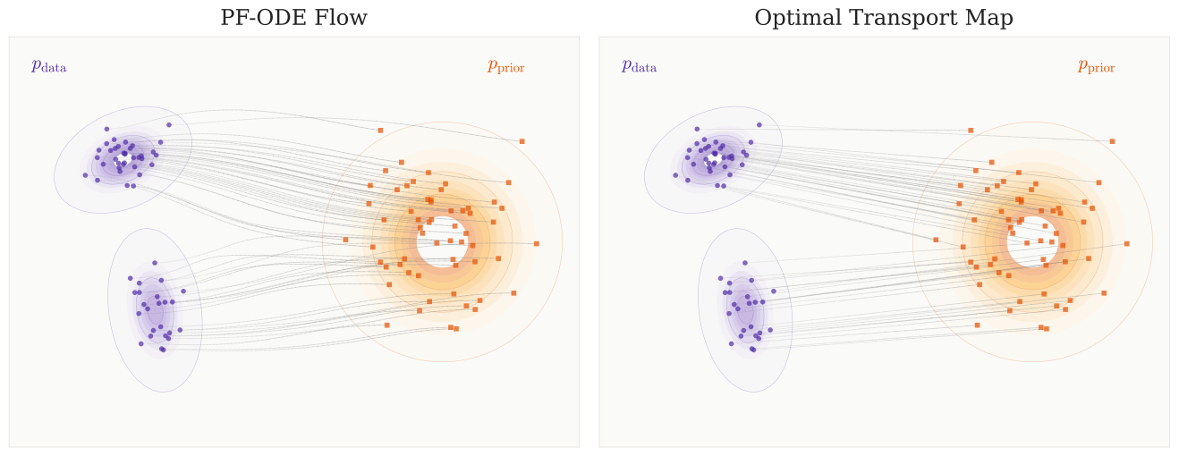
A natural question is whether the deterministic flow map induced by a diffusion process coincides with the optimal transport map under quadratic cost. The answer is no in general, and explicit counterexamples are already available in Gaussian settings. In particular, Tanana (2017) showed that, for a diffusion flow with a more general Gaussian reference, the resulting deterministic transport map can differ from the Brenier optimal transport map even when the endpoint distributions are Gaussian. Since both maps are explicit in this setting, their difference can be verified directly.

Below we present the stronger construction of Lavenant and Santambrogio (2022) in the standard-Gaussian Ornstein–Uhlenbeck setting that is directly relevant to diffusion models. Their argument establishes non-optimality for a broader class of initial distributions and provides structural insight into why the corresponding PF-ODE flow map need not be an optimal transport map.

Setup.

We consider a VP SDE, specifically the Ornstein–Uhlenbeck process, which evolves a smooth initial density \(p_0\) toward the standard Gaussian \(\mathcal{N}(\bm{0}, {\mathbf{I}})\): \[\mathop{}\!\mathrm{d}{\mathbf{x}}(t) = -{\mathbf{x}}(t) \mathop{}\!\mathrm{d}t + \sqrt{2} \mathop{}\!\mathrm{d}{\mathbf{w}}(t), \quad {\mathbf{x}}(0) \sim p_0.\] The associated PF-ODE is given by \[\frac{\mathop{}\!\mathrm{d}\mathbf{S}_t({\mathbf{x}})}{\mathop{}\!\mathrm{d}t} = -\mathbf{S}_t({\mathbf{x}}) - \nabla \log p_t(\mathbf{S}_t({\mathbf{x}})), \quad \mathbf{S}_0({\mathbf{x}}) = {\mathbf{x}}.\] Here, \(\mathbf{S}_t\) denotes the flow map pushing forward \(p_0\) to the marginal \(p_t\): \[\left(\mathbf{S}_t\right) \# p_0 = p_t, \quad\text{that is,}\quad p_t({\mathbf{y}}) = \int_{\mathbb{R}^D} \delta({\mathbf{y}}- \mathbf{S}_t({\mathbf{x}})) p_0({\mathbf{x}}) \mathop{}\!\mathrm{d}{\mathbf{x}}.\] These densities \(p_t\) evolve via the Fokker-Planck equation: \[\frac{\partial p_t}{\partial t} = \nabla \cdot ({\mathbf{x}}p_t) + \Delta p_t.\] This is equivalent to a continuity equation with velocity field: \[{\mathbf{v}}_t({\mathbf{x}}) = -{\mathbf{x}}- \nabla \log p_t({\mathbf{x}}),\] whose flow is given by \(\mathbf{S}_t({\mathbf{x}})\). In other words, the PF-ODE can be written as: \[\frac{\mathop{}\!\mathrm{d}\mathbf{S}_t({\mathbf{x}})}{\mathop{}\!\mathrm{d}t} = {\mathbf{v}}_t\left(\mathbf{S}_t({\mathbf{x}})\right).\]

As \(t \to \infty\), the map transports the initial distribution to the prior: \[\mathbf{S}_\infty \# p_0 = \mathcal{N}(\bm{0}, {\mathbf{I}}) =: p_{\text{prior}}.\]

Objective of Lavenant and Santambrogio (2022)’s Argument.

Lavenant and Santambrogio (2022) do not directly assess whether the terminal map \(\mathbf{S}_\infty\) from \(p_0\) to the Gaussian is optimal. Instead, they construct a specific initial distribution \(p_0\) and examine the entire PF-ODE trajectory. Their key observation is that optimality may fail at some point along the flow.

They consider the intermediate marginal \(p_t = \mathbf{S}_t \# p_0\) and define the residual transport map from \(p_{t_0}\) to the Gaussian as \[\mathbf{T}_{t \to \infty} := \mathbf{S}_\infty \circ \mathbf{S}_{t}^{-1}, \quad \text{for all } t\geq 0.\] The core of their argument shows that, for a carefully chosen \(p_0\), there exists a time \(t_0 \geq 0\) such that \(\mathbf{T}_{t_0 \to \infty}\) is not the quadratic-cost optimal transport map from the new starting distribution \(p_{t_0}\) to \(\mathcal{N}(\bm{0}, {\mathbf{I}})\).

This result demonstrates that PF-ODE flows do not, in general, yield optimal transport maps, and that the property of optimality can break down for certain initial distributions.

Some Tools.

The argument of Lavenant and Santambrogio (2022) crucially relies on the following result, known as Brenier’s theorem:

Let \(\nu_1, \nu_2\) be two probability distributions on \(\mathbb{R}^D\) with smooth densities. A smooth map \({\mathbf{T}}: \mathbb{R}^D \to \mathbb{R}^D\) is the optimal transport from \(\nu_1\) to \(\nu_2\) (under quadratic cost) if and only if \({\mathbf{T}}= \nabla u\) for some convex function \(u\). In this case, \(\mathrm{D} {\mathbf{T}}\) is symmetric and positive semi-definite, and \(u\) satisfies the Monge–Ampère equation: \[\det \mathrm{D}^2 u(\mathbf{x}) = \frac{\nu_1(\mathbf{x})}{\nu_2(\nabla u(\mathbf{x}))}.\]

The proof also implicitly uses the following fact, which we will not repeat each time: a map is the optimal transport between two distributions if and only if its inverse is the optimal transport in the reverse direction.

Proof Sketch: PF-ODE Is Not an OT Map in General.

Lavenant and Santambrogio (2022) employ a proof by contradiction: they assume that for every \(t\ge0\), the map \[\mathbf{T}_t = \mathbf{S}_t \circ \mathbf{S}_\infty^{-1}\] is the quadratic-cost optimal transport map from \(\mathcal{N}(\bm{0},{\mathbf{I}})\) to \(p_t\).

Step 1: Brenier’s Theorem.

By Brenier’s Theorem, the Jacobian of any optimal transport map from Gaussian must be symmetric and positive semi-definite. Thus, \[\mathrm{D} \mathbf{T}_t({\mathbf{x}}) = \mathrm{D} \mathbf{S}_t(\mathbf{S}_\infty^{-1}({\mathbf{x}})) \mathrm{D} (\mathbf{S}_\infty^{-1})({\mathbf{x}})\] must be symmetric for all \(t\) and \({\mathbf{x}}\). Here, \(\mathrm{D} \mathbf{T}_t({\mathbf{x}})\) denotes the total differentiation with respect to \({\mathbf{x}}\).

Step 2: Time-Differentiating the Symmetry Condition.

Differentiating in time: \[\frac{\partial}{\partial t} \mathrm{D}\mathbf{T}_t({\mathbf{x}}) = \left( \frac{\partial}{\partial t} \mathrm{D} \mathbf{S}_t \right)(\mathbf{S}_\infty^{-1}({\mathbf{x}})) \mathrm{D} (\mathbf{S}_\infty^{-1})({\mathbf{x}}).\] Given that the symmetry holds for all \(t\), it follows that this derivative remains symmetric.

Using the flow ODE (differentiating in \({\mathbf{x}}\)), we obtain: \[\frac{\partial (\mathrm{D}\mathbf{S}_t)}{\partial t} = \mathrm{D}{\mathbf{v}}_t(\mathbf{S}_t) \cdot \mathrm{D}\mathbf{S}_t = \left( -{\mathbf{I}}- \mathrm{D}^2 \log p_t(\mathbf{S}_t) \right) \cdot \mathrm{D}\mathbf{S}_t.\] Combining the above, we see that \[\left( -{\mathbf{I}}- \mathrm{D}^2 \log p_t(\mathbf{S}_t) \right) \cdot\mathrm{D}\mathbf{S}_t \cdot \mathrm{D} (\mathbf{S}_\infty^{-1})\] is symmetric for all \(t\geq 0\).

At \(t = 0\), we have \(\mathbf{S}_0 = {\mathbf{I}}\) and \(\mathrm{D}\mathbf{S}_0 = {\mathbf{I}}\), yielding: \[\left( -{\mathbf{I}}- \mathrm{D}^2 \log p_0(\mathbf{S}_\infty^{-1}({\mathbf{x}})) \right) \cdot \mathrm{D} (\mathbf{S}_\infty^{-1})({\mathbf{x}}) \quad \text{is symmetric}.\]

Step 3: The Commutation Condition.

Since \(\mathbf{T}_0 = \mathbf{S}_\infty^{-1}\) is assumed to be optimal, its Jacobian \(D\mathbf{T}_0 = \mathrm{D}(\mathbf{S}_\infty^{-1})\) is symmetric. Moreover, the Hessian \(\mathrm{D}^2\log p_0\) is symmetric. Recall that two symmetric matrices multiply to a symmetric matrix if and only if they commute. Hence, for all \(\mathbf{x}\in\mathbb{R}^D\), \[\mathrm{D}^2\log p_0\bigl(\mathbf{S}_\infty^{-1}(\mathbf{x})\bigr) \quad\text{must commute with}\quad \mathrm{D}(\mathbf{S}_\infty^{-1})(\mathbf{x}) .\] Setting \(\mathbf{y}=\mathbf{S}_\infty^{-1}(\mathbf{x})\) gives the equivalent condition: for all \({\mathbf{y}}\in\mathbb{R}^D\), \[\mathrm{D}^2\log p_0(\mathbf{y}) \quad\text{must commute with}\quad \mathrm{D}\mathbf{S}_\infty(\mathbf{y}) .\]

Now, we transform this condition into a more computable form. Since \(\mathbf{S}_\infty\) is optimal between \(p_0\) and \(\mathcal{N}(\bm{0},{\mathbf{I}})\), Brenier’s theorem guarantees that \(\mathbf{S}_\infty = \nabla u\) for some convex function \(u\). From the Monge–Ampère equation, it follows that: \[\log p_0({\mathbf{y}}) = \log \det(\mathrm{D}^2 u({\mathbf{y}})) - \frac{1}{2} \|\nabla u({\mathbf{y}})\|^2 + \text{Constant}.\] The condition becomes (with \(\mathrm{D}{\mathbf{S}}_\infty = \mathrm{D}^2 u\)):

This yields a necessary condition for \(\mathbf{T}_t\) to be optimal.

Step 4: Constructing the Counterexample.

Let us show how to leverage this necessary condition to derive a contradiction.

Assume we can construct a convex function \(u\) such that \[\mathrm{D}^2 \left( \log \det \mathrm{D}^2 u(\mathbf{x}) - \frac{1}{2} \lvert \nabla u(\mathbf{x}) \rvert^2 \right)\] does not commute with \(\mathrm{D}^2 u(\mathbf{x})\) for some \(\mathbf{x} \in \mathbb{R}^D\). Defining \(p_0 = (\nabla u)^{-1} \# \mathcal{N}(\bm{0}, {\mathbf{I}})\), Brenier’s theorem implies that \(\nabla u\) is the optimal transport from \(p_0\) to \(\mathcal{N}(\bm{0}, {\mathbf{I}})\). However, the condition in Equation \(\eqref{eq:necessary-ot}\) fails, leading to a contradiction. Thus, our goal is to construct such a function. Consider \[u(\mathbf{x}) = \frac{1}{2} \|\mathbf{x}\|^2 + \varepsilon \phi(\mathbf{x}), \quad \text{for a small } \varepsilon.\] Then \(\mathrm{D}^2 u(\mathbf{0}) = {\mathbf{I}}+ \varepsilon \mathrm{D}^2 \phi(\mathbf{0})\), and the commutation condition at \(\mathbf{x} = \mathbf{0}\) requires \(\mathrm{D}^2 \phi(\mathbf{0})\) to commute with \(\mathrm{D}^2 (\Delta \phi)(\mathbf{0})\).

For example, in \(\mathbb{R}^2\), choosing \[\phi(x_1, x_2) = x_1 x_2 + x_1^4\] provides a counterexample where the Hessian \(\mathrm{D}^2 \log p_0\) and the Jacobian \(\mathrm{D}^2 u\) do not commute.

This contradiction shows that \(\mathbf{T}_t\) cannot be optimal for all \(t \geq 0\). Therefore, there exists some \(t_0 \geq 0\) such that the map \(\mathbf{T}_{t_0 \to \infty}\) is not optimal.

Can Canonical Linear Flow and Reflow Leads to an OT Map?

We have seen that the PF-ODE (especially in VP type forward kernel) is generally not an OT map. One natural question now is:

The answer to the question is no.

Nevertheless, combining a linear path with a given coupling offers a practical upper bound on the true OT cost. Among all possible paths, linear interpolation provides the tightest such upper bound, as we will see in the following discussion.

Canonical Linear Flow and Optimal Transport.

Focusing on optimal transport with quadratic cost, we consider the equivalent form of Equation \(\eqref{eq:ot}\), the Benamou–Brenier formulation in Equation \(\eqref{eq:bb-ot}\): \[\begin{equation*} \mathcal{K}\left(p_{\mathrm{src}}, p_{\mathrm{tgt}}\right) := \min_{\substack{ (p_t, {\mathbf{v}}_t) \text{ s.t. } \partial_t p_t + \nabla \cdot (p_t {\mathbf{v}}_t) = 0, \\ p_0 = p_{\mathrm{src}},\,\, p_1 = p_{\mathrm{tgt}} }} \int_0^1 \int_{\mathbb{R}^D} \|{\mathbf{v}}_t({\mathbf{x}})\|^2 p_t({\mathbf{x}}) \mathop{}\!\mathrm{d}{\mathbf{x}}\mathop{}\!\mathrm{d}t. \end{equation*}\] Unlike the static Monge formulation (Equation \(\eqref{eq: Monge's Formulation}\)), where computing the optimal map requires solving the Monge–Ampère equation (Equation \(\eqref{eq:monge-ampere}\)), the Benamou–Brenier problem admits a convex reformulation after introducing the momentum field \({\mathbf{m}}_t := p_t {\mathbf{v}}_t\). Nevertheless, discretizing this convex problem on a grid in \(\mathbb{R}^D\) remains intractable in high dimensions.

While solving the Benamou-Brenier formulation is generally intractable, Liu (2022; Lipman et al. 2024) reveal that its kinetic energy admits a practical upper bound. This is achieved by restricting the search to a simpler family of conditional flows, where each path is defined by its fixed endpoints \(({\mathbf{x}}_0, {\mathbf{x}}_1)\) drawn from a coupling \(\pi_{0,1}\) of the source and target distributions. Within this conditional flow family, the canonical linear interpolation emerges as the optimal choice, as formalized below.

In other words, the linear interpolation \(\bm{\Psi}^*_t\) (i.e., the forward kernel used by Flow Matching and Rectified Flow) minimizes an upper bound on the true kinetic energy for any chosen coupling \(\pi_{0,1}\).

We emphasize that optimality within this class of conditional flows does not guarantee global optimality on the marginal distributions.

Reflow and Optimal Transport.

The most naive transport plan between two distributions is to connect their samples with straight lines using a simple independent coupling. However, this approach is demonstrably not optimal, as the failure lies not in the straight-line paths themselves, but in the inefficient initial pairing of points.

The Reflow procedure may offer a constructive response. It is an iterative algorithm designed specifically to correct this pairing, and crucially, each step is guaranteed to be cost-non-increasing (Liu et al. 2022). This property suggests Reflow systematically pushes the transport plan towards a more optimal configuration, which naturally motivates the central question of its convergence.

The short answer is no in general. Below, we explain what may go wrong. To recall, the Reflow procedure iteratively refines the coupling between \(p_{\mathrm{src}}\) and \(p_{\mathrm{tgt}}\) via the update: \[\pi^{(k+1)} = \texttt{Rectify}(\pi^{(k)}),\] initialized with the product coupling \(\pi^{(0)} := p_{\mathrm{src}}({\mathbf{x}}_0) p_{\mathrm{tgt}}({\mathbf{x}}_1)\). More precisely, \(\texttt{Rectify}\) output the updated coupling \(\pi^{(k+1)}\) via the following: At each iteration \(k = 0, 1, 2, \ldots\), a velocity field \({\mathbf{v}}_t^{(k)}\) is learned via: \[{\mathbf{v}}_t^{(k)} \in \mathop{\mathrm{arg\,min}}_{{\mathbf{u}}_t} \, \mathcal{L}({\mathbf{u}}_t\big\vert\pi^{(k)}),\] where \(\mathcal{L}({\mathbf{u}}_t\big\vert\pi^{(k)})\) is the loss (e.g., RF or FM loss) defined in Equation in Chapter 5. Here, for notational simplicity, we adopt a non-parametric formulation for the velocity field, rather than a parameterized form \(\bm{\phi}\) employed in other contexts. The updated coupling is then given by: \[\pi^{(k+1)}({\mathbf{x}}_0, {\mathbf{x}}_1) := p_{\mathrm{src}}({\mathbf{x}}_0)\, \delta\big({\mathbf{x}}_1 - \bm{\Psi}_1^{(k)}({\mathbf{x}}_0)\big),\] where \(\bm{\Psi}_1^{(k)}\) denotes the solution map at time \(t=1\) obtained by integrating \({\mathbf{v}}_t^{(k)}\) from initial condition \({\mathbf{x}}_0\).

It has been observed in (Liu et al. 2022) that for a coupling \(\pi\) between \(p_{\mathrm{src}}\) and \(p_{\mathrm{tgt}}\), the existence of a velocity field \({\mathbf{v}}_t\) that minimizes the Reflow loss, that is, satisfies \(\mathcal{L}({\mathbf{v}}_t |\pi) = 0\), does not necessarily imply that the transport is optimal.

Motivated by the Benamou–Brenier framework, where the optimal transport velocity is known to be the gradient of a potential function, Liu (2022) proposed an additional constraint: the velocity field \({\mathbf{v}}_t\) should be a potential field. Accordingly, the objective in Equation in Chapter 5 is modified to restrict \({\mathbf{v}}_t\) to the space of gradient vector fields, also known as potential flows: \[\begin{align} \label{eq:reflow-loss-gradient} {\mathbf{w}}_t^{(k)} \in \mathop{\mathrm{arg\,min}}_{\substack{{\mathbf{u}}_t:\, {\mathbf{u}}_t=\nabla\varphi \\ \text{for some }\varphi\colon\mathbb{R}^D\to\mathbb{R}}} \, \mathcal{L}({\mathbf{u}}_t\big\vert\pi^{(k)}), \end{align}\] with the rest of the procedure remaining the same as in Rectify. We denote this associated operator as \(\texttt{Rectify}_{\perp}\), emphasizing the projection onto irrotational vector fields.

Let \(\pi\) be a coupling between \(p_{\mathrm{src}}\) and \(p_{\mathrm{tgt}}\). Liu et al. (2022) conjecture the following equivalence characterizing optimality:

1. \(\pi\) is an optimal transport coupling.

2. \(\pi\) is a fixed point of the potential rectification operator: \[\pi = \texttt{Rectify}_{\perp}(\pi).\]

3. There exists a gradient velocity field \({\mathbf{v}}_t = \nabla \varphi_t\) such that the rectify loss vanishes: \[\mathcal{L}({\mathbf{v}}_t |\pi) = 0.\]

However, Hertrich et al. (2025) exhibit two types of counterexamples:

1. When the intermediate distributions \(p_t\) have disconnected support, one can find fixed points of \(\texttt{Rectify}_{\perp}\) with zero Reflow loss and gradient velocity fields that nonetheless fail to produce the optimal coupling.

2. Even when both endpoint distributions are Gaussian, there exist couplings whose loss is arbitrarily small but whose deviation from the optimal coupling is arbitrarily large.

Therefore, while rectified flows may yield strong generative models, their reliability as optimal transport solvers remains limited. This highlights an important gap between generative modeling and principled optimal transport theory, inviting further research at their intersection.

Finally, we note that transport cost does not always correlate with downstream performance; as such, computing the exact optimal transport map may not necessarily lead to better practical outcomes. Nonetheless, variants of optimal transport remain fundamental to many problems in science and engineering. Diffusion models offer a powerful framework for exploring these challenges.

Closing Remarks

In this chapter, we revisited the classical problem of transporting one distribution to another through the lens of optimal transport and its entropic variants. We reviewed optimal transport in both its static Monge–Kantorovich form and its dynamic Benamou–Brenier formulation, where transport is realized by a deterministic flow minimizing kinetic cost. We then discussed entropy-regularized optimal transport and the Schrödinger bridge (SB), which replace deterministic transport by the most likely controlled diffusion relative to a reference process. From this perspective, diffusion models lie naturally near the SB viewpoint on the stochastic side, while their PF-ODEs define deterministic transport maps on the ODE side. As we emphasized, however, the PF-ODE transport is generally not the quadratic-cost optimal transport map: it is one deterministic coupling among many, rather than the minimizer of the Benamou–Brenier action.

This also highlights a more basic question: before asking whether a transport is optimal, when can two distributions be connected by a deterministic map at all? In many settings, existence is not the main difficulty. Under mild regularity assumptions, one can often find a measurable map \({\mathbf{T}}\) such that \({\mathbf{T}}_\# p_{\mathrm{src}} = p_{\mathrm{tgt}}\). The harder issue is that, beyond one dimension, relatively few classical constructions are both explicit and robust in practice. In one dimension, the monotone rearrangement gives a simple answer by matching quantiles. In higher dimensions, several important constructions are known: Brenier’s theorem (Item) yields the quadratic-cost optimal map under suitable regularity; the Knothe–Rosenblatt rearrangement (Rosenblatt 1952; Knothe 1957) builds a triangular map from iterated conditional distributions; and the Dacorogna–Moser approach (Dacorogna and Moser 1990) constructs smooth diffeomorphic transports through a velocity field solving a divergence equation. Each gives a principled route to deterministic transport, but each also relies on structural assumptions or nontrivial analytical machinery.

From this viewpoint, diffusion-based flow maps provide an appealing and flexible alternative. Rather than prescribing a closed-form transport map, diffusion models and flow-matching methods learn a time-dependent vector field whose induced flow pushes a simple source distribution toward the target. This learned map need not coincide with the Brenier map or any other classical canonical construction, and in general it does not solve a prescribed optimal transport problem. Nevertheless, it offers a practical and expressive route to map-based sampling in high dimensions, where explicit transport-map constructions are often unavailable or difficult to compute. In this sense, diffusion flows are best understood not as replacements for classical transport theory, but as modern learned transport mechanisms that sit alongside optimal transport maps, triangular rearrangements, and PDE-based constructions within the broader landscape of deterministic transport.