Chapter 6: A Unified and Systematic Lens on Diffusion Models
Mathematics is the art of giving the same name to different things.
Henri Poincaré
This chapter presents a systematic viewpoint that connects the variational, score-based, and flow-based perspectives within a coherent picture. Although motivated by different intuitions, these approaches converge on the same core mechanism underlying modern diffusion models: define a forward corruption process that traces a path of marginal distributions, then learn the local quantities needed to construct generative dynamics that follow this path in reverse. Building on Chapter 2, Chapter 3, Chapter 4, and Chapter 5, we observe a common recipe: define a forward corruption process that traces a path of marginals, then learn a time varying vector field that transports a simple prior to the data distribution along this path.
A key ingredient across all perspectives is the conditioning trick introduced in Section 1.1, which transforms an intractable marginal objective into a tractable conditional one, leading to stable and efficient training.
In Section 1.2 we analyze the training objective in a systematic way, identifying its essential components and clarifying how loss functions are formulated in the variational, score-based, and flow-based viewpoints.
Section 1.3 shows that any affine forward noise injection of the form \({\mathbf{x}}_t = \alpha_t {\mathbf{x}}_0 + \sigma_t {\bm{\epsilon}}\) can be equivalently transformed into the standard linear schedule \({\mathbf{x}}_t = (1 - t){\mathbf{x}}_0 + t{\bm{\epsilon}}\). Moreover, common parameterizations such as noise prediction, clean data prediction, score prediction, and velocity prediction are interchangeable at the level of gradients. Thus, the choices of noise schedulers and parameterizations both adhere to the same modeling principle.
Finally, Section 1.4 brings the discussion together and identifies the governing rule: the Fokker–Planck equation. Whether viewed as a variational scheme (discrete time denoising), a score-based method (SDE formulation), or a flow-based method (ODE formulation), each constructs a generator whose marginals follow the same density evolution. The Fokker–Planck equation thus serves as the universal constraint respected by all three viewpoints, with differences arising only in parameterization and training objectives.
After this chapter, you will be able to...
recognize the common conditioning principle behind variational, score-based, and flow-based training: an intractable marginal target can be learned through tractable conditional targets;
understand the four common prediction types—clean data, noise, score, and velocity—and convert between their oracle predictions when the forward schedule is nondegenerate;
disentangle the main design choices in diffusion training: the forward noise schedule, prediction target, time-sampling distribution, and time weighting, and understand which changes are mathematical reparameterizations and which can still affect practical optimization;
distinguish different notions of “equivalence”: representing the same oracle information, having equivalent population objectives up to weighting or additive constants, tracing the same marginal density path, and behaving identically as a practical training or sampling algorithm;
understand how different affine probability paths are related through time reparameterization and spatial rescaling, while keeping track of what these transformations do and do not preserve;
understand how the continuity and Fokker–Planck equations provide the density-level principle connecting variational, deterministic ODE, and stochastic SDE descriptions of diffusion models.
Reader route. This chapter is the conceptual keystone of the book. For a first pass, focus on the conditioning principle, the relationships among the four prediction types, and the continuity/Fokker–Planck view that connects the three perspectives. The central lesson is not to memorize every conversion formula, but to ask what notion of equivalence is being used and what that equivalence actually preserves. The detailed analysis of weighting, schedules, and parameterization choices can then be revisited to understand why mathematically equivalent formulations may still behave differently in practice.
Conditional Tricks: The Secret Sauce of Diffusion Models
Until now, we have explored diffusion models from three seemingly distinct origins: variational, score-based, and flow based perspectives. Each was originally motivated by different goals and led to its own training objectives (with a fixed \(t\)):
Variational View: Learn a parametrized density \(p_{\bm{\phi}}(\mathbf{x}_{t-\Delta t}|\mathbf{x}_t)\) to approximate the oracle reverse transition \(p(\mathbf{x}_{t-\Delta t}|\mathbf{x}_t)\) by minimizing: \[\mathcal{J}_{\text{KL}}(\bm{\phi}) := \mathbb{E}_{p_t(\mathbf{x}_t)}\left[ \mathcal{D}_{\mathrm{KL}}\big(p(\mathbf{x}_{t-\Delta t}|\mathbf{x}_t) \| p_{\bm{\phi}}(\mathbf{x}_{t-\Delta t}|\mathbf{x}_t)\big) \right];\]
Score-Based View: Learn a score model \({\mathbf{s}}_{\bm{\phi}}({\mathbf{x}}_t, t)\) to approximate the marginal score \(\nabla_{{\mathbf{x}}} \log p_t({\mathbf{x}}_t)\) via: \[\mathcal{J}_{\text{SM}}(\bm{\phi}) := \mathbb{E}_{p_t({\mathbf{x}}_t)}\left[ \left\| {\mathbf{s}}_{\bm{\phi}}({\mathbf{x}}_t, t) - \nabla_{{\mathbf{x}}} \log p_t({\mathbf{x}}_t) \right\|_2^2 \right];\]
Flow-Based View: Learn a velocity model \({\mathbf{v}}_{\bm{\phi}}({\mathbf{x}}_t, t)\) to match the oracle velocity \({\mathbf{v}}_t({\mathbf{x}}_t)\) (e.g., defined by Equation in Chapter 5) by minimizing: \[\mathcal{J}_{\text{FM}}(\bm{\phi}) := \mathbb{E}_{p_t({\mathbf{x}}_t)} \left[ \left\| {\mathbf{v}}_{\bm{\phi}}({\mathbf{x}}_t, t) - {\mathbf{v}}_t({\mathbf{x}}_t) \right\|_2^2 \right].\]
At first glance, these objectives seem hopelessly intractable, since they all require access to oracle quantities that are fundamentally unknowable in general. But here comes the exciting twist: each method independently arrives at the same elegant solution to this problem: conditioning on the data \({\mathbf{x}}_0\). This technique transforms each intractable training target into a tractable one.
This elegant “conditioning technique” rewrites the objectives as expectations over the known Gaussian conditionals \(p_t({\mathbf{x}}_t | {\mathbf{x}}_0)\), yielding tractable conditional targets and training objectives that are gradient-equivalent to their marginal counterparts:
Variational View (Equation in Chapter 2): \[\mathcal{J}_{\text{KL}}(\bm{\phi}) = \underbrace{\mathbb{E}_{{\mathbf{x}}_0} \mathbb{E}_{p_t({\mathbf{x}}_t|{\mathbf{x}}_0)} \left[ \mathcal{D}_{\mathrm{KL}}\big(p({\mathbf{x}}_{t-\Delta t}|{\mathbf{x}}_t, {\mathbf{x}}_0) \| p_{\bm{\phi}}({\mathbf{x}}_{t-\Delta t}|{\mathbf{x}}_t)\big) \right]}_{\mathcal{J}_{\text{CKL}}(\bm{\phi})} + C;\]
Score-Based View (Equation in Chapter 3): \[\mathcal{J}_{\text{SM}}(\bm{\phi}) = \underbrace{\mathbb{E}_{{\mathbf{x}}_0} \mathbb{E}_{p_t({\mathbf{x}}_t|{\mathbf{x}}_0)} \left[ \left\| {\mathbf{s}}_{\bm{\phi}}({\mathbf{x}}_t, t) - \nabla_{{\mathbf{x}}_t} \log p_t({\mathbf{x}}_t | {\mathbf{x}}_0) \right\|_2^2 \right]}_{\mathcal{J}_{\text{DSM}}(\bm{\phi})} + C;\]
Flow-Based View (Equation in Chapter 5): \[\mathcal{J}_{\text{FM}}(\bm{\phi}) = \underbrace{\mathbb{E}_{{\mathbf{x}}_0} \mathbb{E}_{p_t({\mathbf{x}}_t|{\mathbf{x}}_0)} \left[ \left\| {\mathbf{v}}_{\bm{\phi}}({\mathbf{x}}_t, t) - {\mathbf{v}}_t({\mathbf{x}}_t | {\mathbf{x}}_0) \right\|^2 \right]}_{\mathcal{J}_{\text{CFM}}(\bm{\phi})} + C.\]
To build a unified view, we next revisit the conditional KL, score, and velocity objectives in a systematic manner. Crucially, these objectives are not only tractable but also equivalent to their original forms up to a constant vertical shift. The conditional versions (\(\mathcal{J}_{\text{CKL}}\), \(\mathcal{J}_{\text{DSM}}\), \(\mathcal{J}_{\text{CFM}}\)) differ from the originals (\(\mathcal{J}_{\text{KL}}\), \(\mathcal{J}_{\text{SM}}\), \(\mathcal{J}_{\text{FM}}\)) only by a constant that is independent of the model parameters. Consequently, each conditional objective has the same minimizers as its original counterpart within the same model class.
To see what these minimizers ideally recover, suppose the model is expressive enough to represent the exact oracle. Despite their different objectives, all three perspectives then share the same conceptual pattern: \[\underbrace{\text{marginal oracle}}_{\text{generally intractable}} = \mathbb{E}_{{\mathbf{x}}_0\sim p(\cdot|{\mathbf{x}}_t)} \left[ \underbrace{\text{conditional oracle}}_{\text{tractable given }{\mathbf{x}}_0} \right].\] That is, conditioning on the clean sample \({\mathbf{x}}_0\) gives a tractable target, and averaging these conditional targets over the possible clean samples consistent with \({\mathbf{x}}_t\) recovers the desired marginal oracle. Concretely,
\[\begin{align} \label{eq:three-minimizer-oracle} \begin{aligned} p^*(\mathbf{x}_{t-\Delta t}|\mathbf{x}_t) &= \mathbb{E}_{\mathbf{x}_0 \sim p(\cdot|\mathbf{x}_t)} \big[p(\mathbf{x}_{t-\Delta t}|\mathbf{x}_t, \mathbf{x}_0)\big] &&= p(\mathbf{x}_{t-\Delta t}|\mathbf{x}_t), \\ \mathbf{s}^*(\mathbf{x}_t, t) &= \mathbb{E}_{\mathbf{x}_0 \sim p(\cdot|\mathbf{x}_t)} \big[\nabla_{\mathbf{x}_t} \log p_t(\mathbf{x}_t|\mathbf{x}_0)\big] &&= \nabla_{\mathbf{x}_t} \log p_t(\mathbf{x}_t), \\ \mathbf{v}^*(\mathbf{x}_t, t) &= \mathbb{E}_{\mathbf{x}_0 \sim p(\cdot|\mathbf{x}_t)} \big[\mathbf{v}_t(\mathbf{x}_t|\mathbf{x}_0)\big] &&= \mathbf{v}_t(\mathbf{x}_t). \end{aligned} \end{align}\]
For the variational view, the first identity follows from marginalizing the conditional reverse transition over \({\mathbf{x}}_0\), and the KL objective is minimized by the resulting marginal reverse transition. For score and velocity matching, the squared-error objectives are least-squares regressions whose population minimizers are the corresponding conditional expectations. These identities describe the unrestricted population oracles; a restricted neural model need not represent them exactly. Below is a concrete example of a scenario with a finite number of data points.
Example: Closed-Form Oracle Targets on a Finite Dataset
To make Equation \(\eqref{eq:three-minimizer-oracle}\) more concrete, suppose the data distribution is the empirical measure \[\hat p_0=\frac{1}{N}\sum_{i=1}^N \delta_{{\mathbf{x}}_0^{(i)}},\] where \(\{{\mathbf{x}}_0^{(i)}\}_{i=1}^N\) denotes the finite training set.
In Equation \(\eqref{eq:three-minimizer-oracle}\), the notation \[{\mathbf{x}}_0 \sim p(\cdot|{\mathbf{x}}_t)\] means that we average over the posterior distribution of the clean sample given the noisy observation \({\mathbf{x}}_t\). Equivalently, for any quantity \({\mathbf{h}}({\mathbf{x}}_0)\), \[\mathbb{E}_{{\mathbf{x}}_0 \sim p(\cdot|{\mathbf{x}}_t)}[{\mathbf{h}}({\mathbf{x}}_0)] = \int {\mathbf{h}}({\mathbf{x}}_0)\, p({\mathbf{x}}_0|{\mathbf{x}}_t)\mathop{}\!\mathrm{d}{\mathbf{x}}_0.\]
By Bayes’ rule, \[p({\mathbf{x}}_0|{\mathbf{x}}_t) = \frac{p_t({\mathbf{x}}_t|{\mathbf{x}}_0)\,p_{\text{data}}({\mathbf{x}}_0)} {\int p_t({\mathbf{x}}_t|\tilde{{\mathbf{x}}}_0)\,p_{\text{data}}(\tilde{{\mathbf{x}}}_0)\mathop{}\!\mathrm{d}\tilde{{\mathbf{x}}}_0}.\] Under the standard Gaussian diffusion forward process, \[p_t({\mathbf{x}}_t|{\mathbf{x}}_0^{(i)}) = \mathcal{N}\left({\mathbf{x}}_t;\alpha_t {\mathbf{x}}_0^{(i)}, \sigma_t^2 {\mathbf{I}}\right),\] so the conditional likelihood is explicit. However, at the population level, the posterior \(p({\mathbf{x}}_0|{\mathbf{x}}_t)\) still requires averaging over the full data distribution \(p_{\text{data}}\).
If we now replace \(p_{\text{data}}\) by the empirical measure \[\hat p_0=\frac{1}{N}\sum_{i=1}^N \delta_{{\mathbf{x}}_0^{(i)}},\] then the posterior \(p({\mathbf{x}}_0|{\mathbf{x}}_t)\) is supported only on the training examples, and its mass at \({\mathbf{x}}_0^{(i)}\) is \[p({\mathbf{x}}_0={\mathbf{x}}_0^{(i)}|{\mathbf{x}}_t) = \frac{p_t({\mathbf{x}}_t|{\mathbf{x}}_0^{(i)})} {\sum_{j=1}^N p_t({\mathbf{x}}_t|{\mathbf{x}}_0^{(j)})} =: w_i({\mathbf{x}}_t,t), \qquad \sum_{i=1}^N w_i({\mathbf{x}}_t,t)=1.\] Hence the posterior expectation above reduces to the finite sum \[\mathbb{E}_{{\mathbf{x}}_0 \sim p(\cdot|{\mathbf{x}}_t)}[{\mathbf{h}}({\mathbf{x}}_0)] = \sum_{i=1}^N w_i({\mathbf{x}}_t,t){\mathbf{h}}({\mathbf{x}}_0^{(i)}).\] Thus, in the finite-dataset case, the abstract posterior averaging in Equation \(\eqref{eq:three-minimizer-oracle}\) becomes a concrete weighted average over the training set, with weights \(w_i({\mathbf{x}}_t,t)\). We now make these three cases explicit.
Variational View.
The oracle reverse transition becomes \[p^*({\mathbf{x}}_{t-\Delta t}|{\mathbf{x}}_t) = \sum_{i=1}^N w_i({\mathbf{x}}_t,t) p({\mathbf{x}}_{t-\Delta t}|{\mathbf{x}}_t,{\mathbf{x}}_0^{(i)}).\] Here each conditional reverse kernel \[p({\mathbf{x}}_{t-\Delta t}|{\mathbf{x}}_t,{\mathbf{x}}_0^{(i)})\] is itself available in closed form under Gaussian diffusion; in fact, it is Gaussian as shown in Lemma in Chapter 2 (Reverse Conditional Transition Kernel). So the true reverse kernel is simply a posterior-weighted mixture of explicit Gaussian bridges.
Score-Based View.
Likewise, the oracle score becomes \[\mathbf{s}^*({\mathbf{x}}_t,t) = \sum_{i=1}^N w_i({\mathbf{x}}_t,t) \nabla_{{\mathbf{x}}_t}\log p_t({\mathbf{x}}_t|{\mathbf{x}}_0^{(i)}).\] The conditional score is explicit: \[\nabla_{{\mathbf{x}}_t}\log p_t({\mathbf{x}}_t|{\mathbf{x}}_0^{(i)}) = -\frac{{\mathbf{x}}_t-\alpha_t{\mathbf{x}}_0^{(i)}}{\sigma_t^2}.\] Therefore, \[\mathbf{s}^*({\mathbf{x}}_t,t) = -\frac{1}{\sigma_t^2} \left( {\mathbf{x}}_t-\alpha_t\sum_{i=1}^N w_i({\mathbf{x}}_t,t) {\mathbf{x}}_0^{(i)} \right).\] So the marginal score points from the noisy sample toward a posterior-weighted average of training examples.
Flow-Based View.
The same phenomenon appears for flow matching: \[\mathbf{v}^*({\mathbf{x}}_t,t) = \sum_{i=1}^N w_i({\mathbf{x}}_t,t) \mathbf{v}_t({\mathbf{x}}_t|{\mathbf{x}}_0^{(i)}).\] Again, the building blocks are explicit. The corresponding conditional velocity field has closed form: \[\mathbf{v}_t({\mathbf{x}}_t|{\mathbf{x}}_0^{(i)}) = {\alpha}'_t {\mathbf{x}}_0^{(i)} + \frac{{\sigma}'_t}{\sigma_t}\bigl({\mathbf{x}}_t-\alpha_t{\mathbf{x}}_0^{(i)}\bigr).\] Hence the oracle velocity is also an explicit posterior-weighted average over the dataset.
Taken together, these formulas show that, on a finite dataset, all three oracle targets reduce to explicit posterior-weighted averages of closed-form conditional quantities.
Remark on Memorization.
The formulas above characterize the exact oracle targets induced by the empirical distribution \(\hat p_0\), rather than by the unknown population distribution \(p_{\mathrm{data}}\). If the model learned these empirical targets perfectly at every noise level, and if the reverse process were computed without error, then generation would exactly reproduce the empirical distribution \(\hat p_0\). Since \(\hat p_0\) assigns probability only to the training examples, the generated samples would be drawn from the training set itself. In this idealized sense, perfect fitting of the empirical oracle amounts to memorization.
However, a practically trained diffusion model, need not realize this oracle exactly: it is learned with finite model capacity and finite optimization, and its generated distribution is further affected by model approximation and numerical sampling errors. Therefore, the finite-dataset calculation establishes memorization as an exact empirical solution, but does not imply that every practically trained model necessarily memorizes its training set.
The common conditional reformulation is no coincidence: by making training tractable, it reveals a profound unification. Variational diffusion, score-based SDEs, and flow matching are simply different facets of the same principle. Three perspectives, one insight, elegantly connected. We will continue to explore their equivalence throughout the rest of this chapter.
A Roadmap for Elucidating Training Losses in Diffusion Models
This section builds a systematic view of training losses in diffusion models. In Section 1.2.1, we extend the standard three objectives to a broader set of four parameterizations, showing how they arise from different modeling perspectives. In Section 1.2.2, we then distill these results into a general framework that disentangles the structure of diffusion objectives, laying the groundwork for the equivalence results in Section 1.3.
Four Common Parameterizations in Diffusion Models
Throughout this section, we consider the forward perturbation kernel \[p_t(\mathbf{x}_t|\mathbf{x}_0) = \mathcal{N}\left(\mathbf{x}_t; \alpha_t \mathbf{x}_0, \sigma_t^2 \mathbf{I} \right),\] where \(\mathbf{x}_0 \sim p_{\mathrm{data}}\), as defined in Equation in Chapter 4, unless stated otherwise.
Let \(\omega: [0, T] \to \mathbb{R}_{>0}\) denote a positive time-weighting function. The four standard parameterizations (noise \(\bm{\epsilon}_{\bm{\phi}}\), clean \({\mathbf{x}}_{\bm{\phi}}\), score \({\mathbf{s}}_{\bm{\phi}}\), and velocity \({\mathbf{v}}_{\bm{\phi}}\)), together with their respective minimizers \(\bm{\epsilon}^*\), \({\mathbf{x}}^*\), \({\mathbf{s}}^*\), and \({\mathbf{v}}^*\), are summarized below for clarity and to facilitate further discussion.
Variational View.
Based on the KL divergence in DDPMs (see Section (Practical Choices of Predictions and Loss) in Chapter 2 and Section (Connection to Variational-Based Diffusion Model) in Chapter 4), this approach reduces to predicting either the expected noise that produces \(\mathbf{x}_t\) or the expected clean signal that \(\mathbf{x}_t\) was perturbed from.
\({\bm{\epsilon}}\)-Prediction (Noise Prediction) (Ho et al. 2020): \[\begin{equation} \label{eq:noise-def} \bm{\epsilon}_{\bm{\phi}}(\mathbf{x}_t,t) \approx \mathbb{E}[\bm{\epsilon}|\mathbf{x}_t]=\bm{\epsilon}^*({\mathbf{x}}_t, t) \end{equation}\] with training objective \[\mathcal{L}_{\text{noise}}(\bm{\phi}) := \mathbb{E}_t \left[\omega(t) \mathbb{E}_{\mathbf{x}_0, \bm{\epsilon}} \left\| \bm{\epsilon}_{\bm{\phi}}(\mathbf{x}_t,t) - \bm{\epsilon} \right\|_2^2 \right].\] Here, \({\bm{\epsilon}}^*\) means the average noise that was injected to obtain the given \({\mathbf{x}}_t\).
\({\mathbf{x}}\)-Prediction (Clean Prediction) (Kingma et al. 2021; Karras et al. 2022; Song et al. 2023): \[\begin{equation} \label{eq:clean-def} \mathbf{x}_{\bm{\phi}}(\mathbf{x}_t,t) \approx \mathbb{E}[\mathbf{x}_0|\mathbf{x}_t]={\mathbf{x}}^*({\mathbf{x}}_t, t) \end{equation}\] with training objective \[\mathcal{L}_{\text{clean}}(\bm{\phi}) := \mathbb{E}_t \left[\omega(t) \mathbb{E}_{\mathbf{x}_0, \bm{\epsilon}} \left\| \mathbf{x}_{\bm{\phi}}(\mathbf{x}_t,t) - \mathbf{x}_0 \right\|_2^2 \right].\] Here, \({\mathbf{x}}^*\) means the average of all plausible clean guesses, given the noisy observation \({\mathbf{x}}_t\).
Score-Based View.
Predicts the score function at noise level \(t\), which points in the average direction to denoise \(\mathbf{x}_t\) back toward all possible clean samples that could have generated it:
Score Prediction (Song and Ermon 2019; Song et al. 2020): \[\begin{equation} \label{eq:score-def} \mathbf{s}_{\bm{\phi}}(\mathbf{x}_t,t) \approx \nabla_{\mathbf{x}_t} \log p_t(\mathbf{x}_t) = \mathbb{E}\left[\nabla_{\mathbf{x}_t} \log p_t(\mathbf{x}_t|\mathbf{x}_0) |\mathbf{x}_t\right] = {\mathbf{s}}^*({\mathbf{x}}_t, t) \end{equation}\] with training objective \[\mathcal{L}_{\text{score}}(\bm{\phi}) := \mathbb{E}_t \left[\omega(t) \mathbb{E}_{\mathbf{x}_0, \bm{\epsilon}} \left\| \mathbf{s}_{\bm{\phi}}(\mathbf{x}_t,t) - \nabla_{\mathbf{x}_t} \log p_t(\mathbf{x}_t|\mathbf{x}_0) \right\|_2^2 \right],\] where the conditional score satisfies \(\nabla_{\mathbf{x}_t} \log p_t(\mathbf{x}_t|\mathbf{x}_0) = -\frac{1}{\sigma_t} \bm{\epsilon}\).
Flow-Based View.
Predicts the instantaneous average velocity of the data as it evolves through \(\mathbf{x}_t\):
\({\mathbf{v}}\)-Prediction (Velocity Prediction) (Lipman et al. 2022; Liu 2022; Salimans and Ho 2021; Albergo et al. 2023): \[\begin{equation} \label{eq:velocity-def} \mathbf{v}_{\bm{\phi}}(\mathbf{x}_t, t) \approx \mathbb{E}\left[\left. \frac{\mathop{}\!\mathrm{d}\mathbf{x}_t}{\mathop{}\!\mathrm{d}t} \right| {\mathbf{x}_t}\right] ={\mathbf{v}}^*({\mathbf{x}}_t, t) \end{equation}\] with training objective \[\mathcal{L}_{\text{velocity}}(\bm{\phi}) := \mathbb{E}_t \left[\omega(t) \mathbb{E}_{\mathbf{x}_0, \bm{\epsilon}} \left\| \mathbf{v}_{\bm{\phi}}(\mathbf{x}_t,t) - {\mathbf{v}}_t({\mathbf{x}}_t | {\mathbf{x}}_0,\bm{\epsilon}) \right\|_2^2 \right],\] where the conditional velocity is \({\mathbf{v}}_t({\mathbf{x}}_t|{\mathbf{x}}_0,\bm{\epsilon}) = \alpha_t' \mathbf{x}_0 + \sigma_t' \bm{\epsilon}\).
Here, \({\mathbf{v}}^*\) indicates the average velocity vector passing through the observation point \({\mathbf{x}}_t\).
Building on the insight from Equation \(\eqref{eq:three-minimizer-oracle}\), all four prediction types ultimately aim to approximate a conditional expectation in the form of the average noise, clean data, score, or velocity given an observed \(\mathbf{x}_t\).
Disentangling the Training Objective of Diffusion Models
As shown in Section 1.2.1, the objective functions for the four prediction types commonly share the following template form for diffusion model training:
\[\begin{align} \label{eq:general-dm-loss-D} \begin{aligned} \mathcal{L}(\bm{\phi}):=\mathbb{E}_{{\mathbf{x}}_0, \bm{\epsilon}} \underbrace{\mathbb{E}_{p_{\text{time}}(t)}}_{\substack{\text{time} \\ \text{distribution}}}\Big[ \underbrace{\omega(t)}_{\substack{\text{time} \\ \text{weighting}}}\underbrace{\left\lVert \mathrm{NN}_{\bm{\phi}}({\mathbf{x}}_t, t) - (A_t {\mathbf{x}}_0 + B_t \bm{\epsilon}) \right\rVert_2^2}_{\text{MSE part}}\Big]. \end{aligned} \end{align}\]
Here, to enhance training efficiency and optimize the diffusion model learning pipeline, several key design choices are crucial (Karras et al. 2022; Lu and Song 2024):
Noise schedule in the forward process of \({\mathbf{x}}_t\) via \(\alpha_t\) and \(\sigma_t\);
Prediction types of \(\mathrm{NN}_{\bm{\phi}}\) and their associated regression targets \((A_t {\mathbf{x}}_0 + B_t \bm{\epsilon})\);
Time-weighting function \(\omega(\cdot) \colon [0,T] \to \mathbb{R}_{\geq 0}\);
Time distribution \(p_{\text{time}}\).
We elaborate on these four components here to serve as a roadmap for the discussions in the following sections.
(A) Noise Schedule \(\alpha_t\) and \(\sigma_t\).
Users have the flexibility to choose schedules tailored to their applications, with common examples summarized in Table (Summary of different interpolants) in Chapter 5. Importantly, as we will demonstrate in Equation and Equation, all affine flows of the form \(\mathbf{x}_t = \alpha_t \mathbf{x}_0 + \sigma_t \bm{\epsilon}\) are mathematically equivalent. Specifically, any such interpolation can be converted to the canonical linear schedule (\(\alpha_t = 1 - t\), \(\sigma_t = t\)) or to a trigonometric schedule (\(\alpha_t = \cos t\), \(\sigma_t = \sin t\)) by appropriate time reparametrization and spatial rescaling.
(B) Parameterization \(\mathrm{NN}_{\bm{\phi}}\) and Training Target \(A_t {\mathbf{x}}_0 + B_t \bm{\epsilon}\).
| Regression Target = | \(A_t{\mathbf{x}}_0 + B_t \bm{\epsilon}\) | |
| \(A_t\) | \(B_t\) | |
| Clean | \(1\) | \(0\) |
| Noise | \(0\) | \(1\) |
| Conditional Score | \(0\) | -\(\frac{1}{\sigma_t}\) |
| Conditional Velocity | \(\alpha_t'\) | \(\sigma_t'\) |
There are two choices that are often coupled in diffusion training: what quantity the network directly predicts and which quantity is compared in the training loss. Clean data, noise, score, and velocity can be used for either purpose.
Matched Prediction and Loss.
The common choice, used in Equation \(\eqref{eq:general-dm-loss-D}\), is to train the network directly in the same prediction type that it outputs. Each prediction type then has a corresponding conditional training target of the form \[\text{Regression Target} = A_t{\mathbf{x}}_0+B_t{\bm{\epsilon}},\] where \(A_t\) and \(B_t\) depend on the prediction type and the forward schedule \((\alpha_t,\sigma_t)\). These targets are summarized in Table 1.1.
For example, an \({\mathbf{x}}\)-prediction network is compared with the clean target \({\mathbf{x}}_0\), whereas a \({\mathbf{v}}\)-prediction network is compared with the conditional velocity \[{\mathbf{v}}_t = \alpha_t'{\mathbf{x}}_0+\sigma_t'{\bm{\epsilon}}.\] As shown later in Equation \(\eqref{eq:predictions-equivalence}\), the four prediction types encode the same oracle information and can be converted into one another.
Predicting One Quantity and Evaluating the Loss in Another.
The network output and the quantity used in the loss can also be chosen separately. The network prediction is first converted using the relations in Equation \(\eqref{eq:predictions-equivalence}\), and the loss is then computed against the corresponding target in the converted prediction type.
For example, under the canonical schedule \[{\mathbf{x}}_t=(1-t){\mathbf{x}}_0+t{\bm{\epsilon}},\] suppose the network directly predicts clean data \({\mathbf{x}}_{\bm{\phi}}({\mathbf{x}}_t,t)\). Converting this prediction to velocity gives \[{\mathbf{v}}_{\bm{\phi}}({\mathbf{x}}_t,t) = \frac{{\mathbf{x}}_t-{\mathbf{x}}_{\bm{\phi}}({\mathbf{x}}_t,t)}{t},\] while the conditional velocity target satisfies \[{\mathbf{v}}_t = \frac{{\mathbf{x}}_t-{\mathbf{x}}_0}{t}.\] Therefore, \[\left\| {\mathbf{v}}_{\bm{\phi}}({\mathbf{x}}_t,t)-{\mathbf{v}}_t \right\|_2^2 = \frac{1}{t^2} \left\| {\mathbf{x}}_{\bm{\phi}}({\mathbf{x}}_t,t)-{\mathbf{x}}_0 \right\|_2^2.\] Thus, with the network output fixed as clean prediction, evaluating a velocity loss is exactly equivalent to applying an additional time-dependent weight to the clean-prediction loss. The corresponding relations for general affine schedules and other prediction types are summarized later in Equation \(\eqref{eq:s-e-x-v-equi}\).
Changing the quantity predicted directly by the network has an additional effect. Although the oracle predictions are algebraically convertible, a finite neural network is then trained to represent a different function, with different output scales and parameter gradients. The choice of network prediction can therefore interact with model architecture and optimization, while the choice of loss also controls the relative weighting of prediction errors across noise levels.
For clarity, Equation \(\eqref{eq:general-dm-loss-D}\) uses the matched prediction-and-loss case unless stated otherwise.
(C) Time Distribution \(p_{\text{time}}(t)\).
We next consider how time \(t\), and hence the noise level, is sampled during training. For convenience, define the fixed-time regression loss \[\mathcal{L}_t(\bm{\phi}) := \mathbb{E}_{{\mathbf{x}}_0,{\bm{\epsilon}}} \left[ \left\| \mathrm{NN}_{\bm{\phi}}({\mathbf{x}}_t,t) - \bigl(A_t{\mathbf{x}}_0+B_t{\bm{\epsilon}}\bigr) \right\|_2^2 \right], \qquad {\mathbf{x}}_t=\alpha_t{\mathbf{x}}_0+\sigma_t{\bm{\epsilon}}.\] Then Equation \(\eqref{eq:general-dm-loss-D}\) can be written compactly as \[\mathcal{L}(\bm{\phi}) = \mathbb{E}_{t\sim p_{\text{time}}} \left[ \omega(t)\mathcal{L}_t(\bm{\phi}) \right].\] Thus, if no correction is applied, sampling some times more frequently also gives them more weight in the objective. At the level of the exact expected loss, only the product \(p_{\text{time}}(t)\omega(t)\) matters.
A different use of nonuniform sampling is importance sampling. Suppose the objective above is fixed, but we instead draw times from a proposal \(q_{\text{time}}(t)\). Then \[\mathcal{L}(\bm{\phi}) = \mathbb{E}_{t\sim q_{\text{time}}} \left[ \frac{p_{\text{time}}(t)}{q_{\text{time}}(t)} \omega(t)\mathcal{L}_t(\bm{\phi}) \right],\] provided \(q_{\text{time}}(t)>0\) wherever \(p_{\text{time}}(t)\omega(t)>0\). With this correction, changing \(q_{\text{time}}\) leaves the objective unchanged and changes only its Monte Carlo estimator, for example its variance.
The key distinction is therefore:
| change \(p_{\text{time}}\) in the objective | different weighting, different objective |
| change \(q_{\text{time}}\) \(+\) importance correction | same objective, different estimator |
We therefore keep time sampling and loss weighting conceptually separate. Uniform time sampling makes this distinction less visible because its density contributes only a constant factor, whereas with nonuniform sampling one must specify whether the sampling distribution defines the objective or merely serves as an importance-sampling proposal.
Both uses appear in diffusion-model training. ScoreFlow explicitly uses importance sampling to reduce the variance of a fixed likelihood-weighted objective (Song et al. 2021). VDM and subsequent analyses similarly show that, when the objective is fixed in noise-level coordinates, the noise schedule can act as an importance-sampling distribution (Kingma et al. 2021; Kingma and Gao 2023). EDM (Karras et al. 2022), by contrast, specifies both a nonuniform training distribution over noise levels and a separate loss weighting, whose combination determines the effective training weight.
(D) Time-Weighting Function \(\omega(t)\).
For a fixed \(p_{\text{time}}\), the weighting function \(\omega(t)\) determines the relative contribution of different times to the training objective. Together with the previous paragraph, the effective weighting over time is therefore \(p_{\text{time}}(t)\omega(t)\).
A simple baseline is uniform time sampling with \(\omega(t)\equiv1\), as in the standard simplified \({\bm{\epsilon}}\)-prediction and FM/RF objectives (Ho et al. 2020; Lipman et al. 2022; Liu 2022). Other weightings emphasize different noise regimes and can also carry likelihood or variational interpretations. For example, for the score-matching objective, the likelihood weighting \(\omega(t)=g^2(t)\) yields an upper bound on the negative log-likelihood under suitable regularity conditions (Song et al. 2021). More generally, SNR-dependent weightings provide a common way to redistribute training emphasis across noise levels (Kingma et al. 2021; Kingma and Gao 2023).
Monotonic Weighting and the ELBO-with-Augmentation View.
A useful way to describe the corruption level is through the log signal-to-noise ratio (log-SNR) \[\Lambda_t := \log\frac{\alpha_t^2}{\sigma_t^2}.\] We use \(\Lambda\) for the full log-SNR, distinguishing it from the half-log-SNR coordinate \(\lambda_t=\log(\alpha_t/\sigma_t)=\tfrac12\Lambda_t\) used later in Chapter 9. Since \(\Lambda_t\) decreases as the forward process becomes noisier, after expressing the loss in a common prediction parameterization, let \(w(\Lambda)\) denote the effective weight assigned to each log-SNR level.
A useful result of Kingma and Gao (2023) is that, if \(w(\Lambda)\) is non-increasing in \(\Lambda\) (equivalently, its weight does not decrease as the forward process becomes noisier), then the weighted diffusion objective can be rewritten, up to terms independent of the model parameters, as an average negative ELBO over Gaussian-perturbed data 1.
Thus, monotonic weighting has a concrete probabilistic interpretation: rather than merely emphasizing some noise levels more than others, it can be viewed as averaging variational training over Gaussian-corrupted versions of the data at different corruption strengths.
Conclusion.
For our purposes, the main lesson is that many apparent design choices in diffusion training can be understood through how they reshape the effective weighting over noise levels in the objective. This weighting in turn influences both the optimization landscape in practice and, in special cases such as monotonic weighting, the variational interpretation of the loss.
Equivalence in Diffusion Models
Many formulations of diffusion models look different because they use different prediction types, training objectives, noise schedules, or continuous-time dynamics. In this section, we clarify in what precise sense these formulations can be equivalent at the exact theoretical level, and how their behavior can still differ for learned models in practice.
At the exact or oracle level, several notions of equivalence will appear:
Predictions. Given the noisy observation \({\mathbf{x}}_t\) and the forward schedule, clean-data, noise, score, and velocity oracles contain the same information and can be converted into one another algebraically.
Training Objectives. Squared-error objectives written in different prediction types can differ by positive time-dependent factors while sharing the same pointwise oracle minimizer. These factors determine how strongly different noise levels are weighted during training.
Affine Forward Process. At the particle level, affine forward processes \[{\mathbf{x}}_t=\alpha_t{\mathbf{x}}_0+\sigma_t{\bm{\epsilon}}\] can be related to canonical affine forms through state rescaling and a corresponding canonical coordinate. When this coordinate evolves monotonically with time, the relation also defines a time reparameterization.
Marginal Density Paths. At the density level, different deterministic and stochastic dynamics can produce the same marginal path \(\{p_t\}_{t\in[0,T]}\). Their sample trajectories may differ, while the evolution of \(p_t\) is governed by the corresponding continuity or Fokker-Planck equation.
We develop these connections from prediction to sampling. Section 1.3.1 first relates the four common oracle prediction types and their training losses. Section 1.3.2 then shows how these predictions lead to different expressions of the same oracle PF–ODE. Next, Section 1.3.3 relates affine probability paths to canonical linear and trigonometric forms. Finally, Section 1.3.4 develops additional intuition for the canonical linear schedule and velocity prediction, including their implications for training and numerical integration.
These exact relationships provide a common mathematical foundation, while the practical choices remain meaningful. Finite neural networks may approximate equivalent oracle quantities differently, and loss weighting, optimization, model architecture, and numerical integration can lead to different training and sampling behavior.
Four Prediction Types Are Equivalent
We begin by analyzing the design choices for component (B) in Equation \(\eqref{eq:general-dm-loss-D}\).
We have seen that the four prediction types are not independent choices but different views of the same underlying quantity. For example, noise and clean predictions are directly related (Section (Practical Choices of Predictions and Loss) in Chapter 2), as are score and noise predictions (Section (Multi-Noise Levels of Denoising Score Matching (NCSN)Multi-Noise Levels of Denoising Score Matching (NCSN)) in Chapter 3). This recurring pattern points to a deeper principle: all four parameterizations are algebraically equivalent and can be converted into one another through simple transformations. To make this connection precise, we state the following proposition, illustrated in Figure 1.1, following (Kingma et al. 2021).
Proposition: Equivalence of Parametrizations
Let the optimal predictions minimizing their respective objectives be \[\bm{\epsilon}^*({\mathbf{x}}_t,t) , \quad {\mathbf{x}}^*({\mathbf{x}}_t,t), \quad {\mathbf{s}}^*({\mathbf{x}}_t,t) , \quad {\mathbf{v}}^*({\mathbf{x}}_t,t),\] corresponding to noise, clean, score, and velocity parameterizations. These satisfy the following equivalences: \[\begin{equation} \label{eq:predictions-equivalence} \begin{aligned} \bm{\epsilon}^*({\mathbf{x}}_t,t) &= -\sigma_t {\mathbf{s}}^*({\mathbf{x}}_t,t), \\ {\mathbf{x}}^*({\mathbf{x}}_t,t) &= \frac{1}{\alpha_t} {\mathbf{x}}_t + \frac{\sigma_t^2}{\alpha_t} {\mathbf{s}}^*({\mathbf{x}}_t,t), \\ {\mathbf{v}}^*({\mathbf{x}}_t,t) &= \alpha_t' {\mathbf{x}}^* + \sigma_t' \bm{\epsilon}^* = f(t){\mathbf{x}}_t - \frac{1}{2} g^2(t){\mathbf{s}}^*({\mathbf{x}}_t,t). \end{aligned} \end{equation}\] Here, \(f(t)\) and \(g(t)\) are related to \(\alpha_t\) and \(\sigma_t\) via Lemma in Chapter 4 (Forward Perturbation Kernel ⟺ Linear SDE). Moreover, these minimizers satisfy the identities given in Equation, Equation, Equation, and Equation.
Proof for Proposition. The proof is similar to that of Proposition in Chapter 4 (Minimizer of DSM), which analyzes the global optimum of various matching losses under the DSM objective. See Section (Theoretical Supplement: A Unified and Systematic View on Diffusion Models) in Appendix D for details. ■
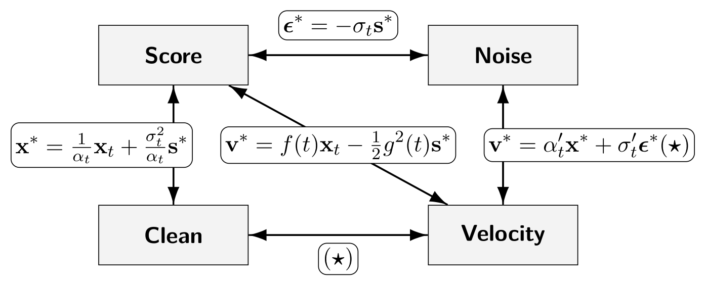
The proposition is most naturally understood as an equivalence of oracle information. At any noise level, knowing one oracle prediction, together with the noisy observation \({\mathbf{x}}_t\) and the forward schedule, determines the others through the identities in Equation \(\eqref{eq:predictions-equivalence}\). For example, the score determines the posterior-mean clean prediction, and either of these determines the PF-ODE velocity. Thus, at the oracle level, these parameterizations contain the same information about the underlying diffusion process.
For a learned model, however, one must distinguish this oracle equivalence from the quantity predicted directly by the neural network. One may choose any of \[\bm{\epsilon}_{\bm{\phi}}({\mathbf{x}}_t,t), \quad {\mathbf{x}}_{\bm{\phi}}({\mathbf{x}}_t,t), \quad {\mathbf{s}}_{\bm{\phi}}({\mathbf{x}}_t,t), \quad {\mathbf{v}}_{\bm{\phi}}({\mathbf{x}}_t,t)\] as the network output. Once one prediction is taken as primary, the others can be defined through the same algebraic conversions as in Equation \(\eqref{eq:predictions-equivalence}\). In particular, for a trained model with parameters \(\bm{\phi}^\times\), these converted predictions are exactly consistent by construction; for example, \[{\mathbf{x}} = \alpha_t {\mathbf{x}}_{\bm{\phi}^\times}({\mathbf{x}},t) + \sigma_t {\bm{\epsilon}}_{\bm{\phi}^\times}({\mathbf{x}},t).\] These conversions are useful both during and after training. For instance, a noise prediction can be converted into a score for reverse-SDE sampling or into a velocity for PF-ODE sampling.
The network prediction parameterization should also be distinguished from the training loss. As discussed in component (B) of Equation \(\eqref{eq:general-dm-loss-D}\), the quantity output by the network need not be the quantity on which the loss is evaluated: the prediction may first be converted into another parameterization before computing the objective. Such a conversion generally changes a squared-error objective by a time-dependent weighting, as shown later in Equation \(\eqref{eq:s-e-x-v-equi}\).
These distinctions matter for finite neural networks. Although the oracle targets are information-equivalent, directly predicting different quantities leads the network to represent and optimize different functions, and the corresponding objectives may weight noise levels differently. Consequently, models trained independently under different prediction parameterizations need not produce identical empirical predictions or identical PF-ODEs. The equivalence in this proposition therefore concerns the information carried by the ideal oracle predictions; the network output parameterization and the training objective remain separate and meaningful design choices.
PF-ODE in Different Parameterizations
The PF-ODE admits several equivalent parameterizations (score, noise, denoised, and velocity). Although interchangeable in principle, the choice has practical consequences: it changes the stiffness of the vector field, the behavior of discretization error, and the ease of optimization. For fast sampling with advanced ODE solvers (see Chapter 9), practitioners often work with \({\bm{\epsilon}}\) or \({\mathbf{x}}\) prediction because they align well with solver inputs and reduce error accumulation. For training generators that use only a few function evaluations (see Chapter 11), \({\mathbf{x}}\) or \({\mathbf{v}}\) prediction often yields smoother objectives and better step to step consistency.
We write the PF-ODE under each parameterization and make the conversions explicit using Equation \(\eqref{eq:predictions-equivalence}\). The results are collected in the following proposition.
Proposition: PF-ODE in Different Parameterizations
Let \(\alpha_t\) and \(\sigma_t\) be the forward perturbation schedules, and denote time derivatives by \(\alpha_t' := \tfrac{\mathop{}\!\mathrm{d}\alpha_t}{\mathop{}\!\mathrm{d}t}\) and \(\sigma_t' := \tfrac{\mathop{}\!\mathrm{d}\sigma_t}{\mathop{}\!\mathrm{d}t}\). Then the empirical PF-ODE admits the equivalent forms \[\begin{align} \label{eq:clean_pf_ode} \begin{aligned} \frac{\mathop{}\!\mathrm{d}{\mathbf{x}}(t)}{\mathop{}\!\mathrm{d}t} &= \frac{\alpha_t'}{\alpha_t} {\mathbf{x}}(t) - \sigma_t \left(\frac{\alpha_t'}{\alpha_t}-\frac{\sigma_t'}{\sigma_t}\right) \bm{\epsilon}^*({\mathbf{x}}(t), t) \\ &= \frac{\sigma_t'}{\sigma_t} {\mathbf{x}}(t) + \alpha_t \left(\frac{\alpha_t'}{\alpha_t}-\frac{\sigma_t'}{\sigma_t}\right) {\mathbf{x}}^*({\mathbf{x}}(t), t) \\ &= \frac{\alpha_t'}{\alpha_t} {\mathbf{x}}(t) + \sigma_t^{2} \left(\frac{\alpha_t'}{\alpha_t}-\frac{\sigma_t'}{\sigma_t}\right) {\mathbf{s}}^*({\mathbf{x}}(t), t) \\ &= \alpha_t'{\mathbf{x}}^*({\mathbf{x}}(t), t) + \sigma_t' {\bm{\epsilon}}^*({\mathbf{x}}(t), t)\\ &= {\mathbf{v}}^*({\mathbf{x}}(t), t). \end{aligned} \end{align}\]
To see the Score SDE notation, we recall Lemma in Chapter 4 (Forward Perturbation Kernel ⟺ Linear SDE). If we set \[f(t) = \frac{\alpha_t'}{\alpha_t}, \quad g^2(t) = \frac{\mathop{}\!\mathrm{d}}{\mathop{}\!\mathrm{d}t} \big(\sigma_t^2\big) - 2 \frac{\alpha_t'}{\alpha_t} \sigma_t^2 = 2\sigma_t\sigma_t' - 2 \frac{\alpha_t'}{\alpha_t} \sigma_t^2,\] then the PF-ODE can be written in the familiar Score SDE form: \[\frac{\mathop{}\!\mathrm{d}{\mathbf{x}}(t)}{\mathop{}\!\mathrm{d}t} = f(t) {\mathbf{x}}(t) - \frac{1}{2} g^2(t) {\mathbf{s}}^*({\mathbf{x}}(t),t).\]
To give a concrete sense of how the PF-ODE is discretized for sampling, we will present in Section (DDIMDDIM) in Chapter 9 the update rule of a widely used diffusion-based ODE sampler, the DDIM scheme. This example will show how an Euler discretization naturally connects with the PF-ODE.
All Affine Flows Are Equivalent
We next analyze the design choices for component (A) in Equation \(\eqref{eq:general-dm-loss-D}\).
State-Level Equivalence.
A convenient canonical interpolation used in FM (Lipman et al. 2022) and RF (Liu 2022) is \[{\mathbf{x}}_t^{\mathrm{FM}}=(1-t) {\mathbf{x}}_0+t {\bm{\epsilon}}= {\mathbf{x}}_{0}+t({\bm{\epsilon}}-{\mathbf{x}}_0),\] whose velocity is the constant vector \({\bm{\epsilon}}-{\mathbf{x}}_0\). The key point of this subsection is that the apparent simplicity of this choice is not essential: any affine interpolation \[{\mathbf{x}}_t=\alpha_t {\mathbf{x}}_0+\sigma_t {\bm{\epsilon}}\] can be written as a time–reparameterized and rescaled version of the canonical path. Define \[c(t):=\alpha_t+\sigma_t, \qquad \tau(t):=\frac{\sigma_t}{\alpha_t+\sigma_t} \quad\big(c(t)\neq 0\big).\] A direct algebraic rewrite yields \[\begin{align*} {\mathbf{x}}_t &=\alpha_t {\mathbf{x}}_0+\sigma_t {\bm{\epsilon}} \\ &=\big(\alpha_t+\sigma_t\big) \left(\frac{\alpha_t}{\alpha_t+\sigma_t}{\mathbf{x}}_0+\frac{\sigma_t}{\alpha_t+\sigma_t}{\bm{\epsilon}}\right) \\ &=c(t) \left(\big(1-\tau(t)\big){\mathbf{x}}_0+\tau(t){\bm{\epsilon}}\right) =c(t) {\mathbf{x}}_{\tau(t)}^{\mathrm{FM}}. \end{align*}\] Hence, whenever \(c(t)\neq0\), every affine path can be represented pointwise as a scalar rescaling of the canonical path. If, in addition, \(\tau(t)\) is continuous and strictly monotone over the time interval of interest, then \(t\mapsto\tau(t)\) is also a genuine change of time variable, and the two paths are related by time reparameterization together with the rescaling \(c(t)\). For the usual forward diffusion schedules, monotonic decay of the signal-to-noise ratio implies monotonic evolution of \(\tau(t)\).
For the associated velocities, apply the chain rule to \({\mathbf{x}}_t=c(t){\mathbf{x}}_{\tau(t)}^{\mathrm{FM}}\): \[\begin{align*} {\mathbf{v}}({\mathbf{x}}_t,t) &:= \frac{\mathop{}\!\mathrm{d}}{\mathop{}\!\mathrm{d}t}\left(\alpha_t{\mathbf{x}}_0 +\sigma_t {\bm{\epsilon}}\right) \\&=\frac{\mathop{}\!\mathrm{d}}{\mathop{}\!\mathrm{d}t}\big(c(t){\mathbf{x}}_{\tau(t)}^{\mathrm{FM}}\big) \\ &=c'(t) {\mathbf{x}}_{\tau(t)}^{\mathrm{FM}}+c(t) \tau'(t) \frac{\mathop{}\!\mathrm{d}}{\mathop{}\!\mathrm{d}s}{\mathbf{x}}^{\mathrm{FM}}_{s}\bigg|_{s=\tau(t)} \\ &=c'(t) {\mathbf{x}}_{\tau(t)}^{\mathrm{FM}}+c(t) \tau'(t) {\mathbf{v}}^{\mathrm{FM}} \left({\mathbf{x}}_{\tau(t)}^{\mathrm{FM}},\tau(t)\right), \end{align*}\] since \({\mathbf{v}}^{\mathrm{FM}}({\mathbf{x}}^{\mathrm{FM}}_{\tau},\tau)=-{\mathbf{x}}_0+{\bm{\epsilon}}\) along the canonical path.
We summarize the above derivation as a formal statement in the following proposition.
Proposition: Equivalence of Affine Flows
Let \({\mathbf{x}}_t^{\mathrm{FM}}=(1-t){\mathbf{x}}_0+t{\bm{\epsilon}}\) and \({\mathbf{x}}_t=\alpha_t{\mathbf{x}}_0+\sigma_t{\bm{\epsilon}}\), with \(c(t):=\alpha_t+\sigma_t\neq 0\) and \(\tau(t):=\sigma_t/(\alpha_t+\sigma_t)\). Then \[\begin{align} \label{eq:fm-general-affine-formula} \begin{aligned} {\mathbf{x}}_t &= c(t){\mathbf{x}}_{\tau(t)}^{\mathrm{FM}}, \\ {\mathbf{v}}({\mathbf{x}}_t,t) &= c'(t){\mathbf{x}}_{\tau(t)}^{\mathrm{FM}} + c(t)\tau'(t) {\mathbf{v}}^{\mathrm{FM}} \left( {\mathbf{x}}_{\tau(t)}^{\mathrm{FM}},\tau(t) \right). \end{aligned} \end{align}\] Thus, every affine interpolation with \(c(t)\neq 0\) admits this canonical state-level representation. When \(\tau(t)\) is additionally continuous and strictly monotone, it can also be interpreted as a time reparameterization together with the scalar rescaling \(c(t)\).
Equivalence with Trigonometric Flow.
Another widely used affine flow is the trigonometric interpolation (Salimans and Ho 2021; Albergo et al. 2023; Lu and Song 2024). As a concrete example, we also show that any affine flow can be expressed in this form. The trigonometric path is defined by \[\begin{align} \label{eq:trig-para} {\mathbf{x}}^{\mathrm{Trig}}_u := \cos(u) {\mathbf{x}}_0 + \sin(u){\bm{\epsilon}}. \end{align}\] Let \(R_t := \sqrt{\alpha_t^2 + \sigma_t^2}\) and assume \(R_t>0\). Choose an angle \(\tau_t\) so that \[\cos \tau_t = \frac{\alpha_t}{R_t}, \qquad \sin \tau_t = \frac{\sigma_t}{R_t}.\] Then every affine interpolation \({\mathbf{x}}_t=\alpha_t{\mathbf{x}}_0+\sigma_t{\bm{\epsilon}}\) admits a pointwise rescaled and re-timed trigonometric path: \[\begin{align} \label{eq:any-to-trig} {\mathbf{x}}_t = \alpha_t{\mathbf{x}}_0+\sigma_t{\bm{\epsilon}} = R_t \left(\frac{\alpha_t}{R_t}{\mathbf{x}}_0+\frac{\sigma_t}{R_t}{\bm{\epsilon}}\right) = R_t {\mathbf{x}}^{\mathrm{Trig}}_{\tau_t}. \end{align}\] The pair \((\alpha_t,\sigma_t)\) is a point in the plane. Normalizing by \(R_t\) places it on the unit circle, which fixes the angle \(\tau_t\) and hence the state \({\mathbf{x}}^{\mathrm{Trig}}_{\tau_t}\); the radius \(R_t\) gives the overall scale. If \(\tau_t\) can additionally be chosen as a continuous and strictly monotone function of \(t\) on the interval of interest, then this state-level representation also defines a genuine time reparameterization.
Differentiating \({\mathbf{x}}^{\mathrm{Trig}}_u\) with respect to \(u\) gives its velocity, \[{\mathbf{v}}^{\mathrm{Trig}}_u = -\sin(u) {\mathbf{x}}_0 + \cos(u) {\bm{\epsilon}}.\] Through the same change of variables as in Equation \(\eqref{eq:any-to-trig}\), this relation provides closed-form conversions for the velocity (and analogously for other parameterizations).
Summarizing the above discussion, we arrive at the following conclusion:
Conclusion
Regardless of the schedule \((\alpha_t,\sigma_t)\), including VE, VP (such as trigonometric), FM, or RF, affine interpolations are mutually convertible by a suitable change of time variable and a scalar rescaling.
Training Objectives of Four Parameterizations.
Let \({\mathbf{x}}_t=\alpha_t {\mathbf{x}}_0+\sigma_t {\bm{\epsilon}}\) with \(\sigma_t>0\) and differentiable \((\alpha_t,\sigma_t)\) such that \(\alpha_t'\sigma_t-\alpha_t\sigma_t'\neq 0\). Consider the oracle targets \[{\bm{\epsilon}}^*({\mathbf{x}}_t,t)=\mathbb{E}[{\bm{\epsilon}}|{\mathbf{x}}_t],\quad {\mathbf{x}}_0^*({\mathbf{x}}_t,t)=\mathbb{E}[{\mathbf{x}}_0|{\mathbf{x}}_t],\quad {\mathbf{v}}^*({\mathbf{x}}_t,t)=\mathbb{E}[\alpha_t'{\mathbf{x}}_0+\sigma_t'{\bm{\epsilon}}|{\mathbf{x}}_t].\] From Proposition: Equivalence of Parametrizations, they satisfy \[\nabla_{{\mathbf{x}}_t}\log p_t({\mathbf{x}}_t) = -\frac{1}{\sigma_t} {\bm{\epsilon}}^*({\mathbf{x}}_t,t) = \frac{\alpha_t}{\sigma_t^2} \left({\mathbf{x}}_0^*({\mathbf{x}}_t,t)-\frac{{\mathbf{x}}_t}{\alpha_t}\right), \quad {\mathbf{v}}^*=\alpha_t' {\mathbf{x}}_0^*+\sigma_t' {\bm{\epsilon}}^*.\] Under the head conversions \[{\mathbf{s}}_{{\bm{\phi}}} \equiv -\frac{1}{\sigma_t} {\bm{\epsilon}}_{{\bm{\phi}}} \equiv \frac{\alpha_t}{\sigma_t^2} \left({\mathbf{x}}_{{\bm{\phi}}}-\frac{{\mathbf{x}}_t}{\alpha_t}\right),\] and the velocity-to-score conversion is \[{\mathbf{s}}_{{\bm{\phi}}} = \frac{\alpha_t}{\sigma_t(\alpha_t'\sigma_t-\alpha_t\sigma_t')} {\mathbf{v}}_{{\bm{\phi}}} - \frac{\alpha_t'}{\sigma_t(\alpha_t'\sigma_t-\alpha_t\sigma_t')} {\mathbf{x}}_t,\] the per–sample squared losses match up to time–dependent weights: \[\begin{align} \label{eq:s-e-x-v-equi} \begin{aligned} \big\|{\mathbf{s}}_{{\bm{\phi}}}-\nabla_{{\mathbf{x}}_t}\log p_t({\mathbf{x}}_t)\big\|_2^2 &=\frac{1}{\sigma_t^2} \big\|{\bm{\epsilon}}_{{\bm{\phi}}}-{\bm{\epsilon}}^*\big\|_2^2 \\ &=\frac{\alpha_t^2}{\sigma_t^4} \big\|{\mathbf{x}}_{{\bm{\phi}}}-{\mathbf{x}}_0^*\big\|_2^2 \\ &=\left(\frac{\alpha_t}{\sigma_t(\alpha_t'\sigma_t-\alpha_t\sigma_t')}\right)^{ 2} \big\|{\mathbf{v}}_{{\bm{\phi}}}-{\mathbf{v}}^*\big\|_2^2 . \end{aligned} \end{align}\]
By Proposition: Equivalence of Affine Flows, any affine flow \({\mathbf{x}}_t=\alpha_t{\mathbf{x}}_0+\sigma_t{\bm{\epsilon}}\) is transferable to the canonical FM path via \({\mathbf{x}}_t=c(t){\mathbf{x}}^{\mathrm{FM}}_{\tau(t)}\) with \(c(t)=\alpha_t+\sigma_t\) and \(\tau(t)=\sigma_t/(\alpha_t+\sigma_t)\). Differentiating gives \[{\mathbf{v}}_{{\bm{\phi}}}({\mathbf{x}}_t,t)=c'(t){\mathbf{x}}^{\mathrm{FM}}_{\tau(t)} +c(t)\tau'(t){\mathbf{v}}^{\mathrm{FM}}_{{\bm{\phi}}} \left({\mathbf{x}}_{\tau(t)}^{\mathrm{FM}},\tau(t)\right), \qquad {\mathbf{x}}_{\tau(t)}^{\mathrm{FM}}=\frac{{\mathbf{x}}_t}{c(t)},\] and the same relation holds for \({\mathbf{v}}^*\). Hence the velocity loss transforms by \[\begin{align*} \big\|{\mathbf{v}}_{{\bm{\phi}}}({\mathbf{x}}_t,t)-{\mathbf{v}}^*({\mathbf{x}}_t,t)\big\|_2^2 = \big(c(t) \tau'(t)\big)^2 \Big\|{\mathbf{v}}^{\mathrm{FM}}_{{\bm{\phi}}} \left(\frac{{\mathbf{x}}_t}{c(t)},\tau(t)\right) -\big({\mathbf{v}}^{\mathrm{FM}}\big)^* \left(\frac{{\mathbf{x}}_t}{c(t)},\tau(t)\right)\Big\|_2^2. \end{align*}\]
With the above observation, we arrive at the following conclusion:
Conclusion
Score, noise, clean, and velocity training objectives are theoretically equivalent up to time–dependent weights (and, for velocity, an affine head conversion involving \({\mathbf{x}}_t\)) determined by \((\alpha_t,\sigma_t)\).
(Optional) Analysis of Parametrizations and the Canonical Flow
Even though we have shown in the previous sections that all four parameterizations are mathematically equivalent and can be transformed into one another, and that the forward affine noise-injection flow is equivalent to the canonical form \[{\mathbf{x}}_t^{\mathrm{FM}} = (1-t) {\mathbf{x}}_0 + t {\bm{\epsilon}},\] in this subsection we provide further intuition and analyze the potential advantages of using the \({\mathbf{v}}\)-prediction parameterization together with this canonical affine flow.
This subsection asks a simple question: how do different parameterizations and schedules shape what the model learns and how we sample? We proceed in two conceptual perspectives:
Regression Targets and Schedules. We focus on why combining \({\mathbf{v}}\)-prediction with the canonical linear schedule \((\alpha_t,\sigma_t)=(1-t,t)\) is natural: it keeps the conditional velocity target scale constant in time and removes the explicit schedule-curvature terms from the velocity decomposition.
Solver Implications. We examine how this parameterization interacts with numerical integration, while deferring the detailed solver analysis to Chapter 9.
Before proceeding, we distinguish between two types of velocity fields to avoid ambiguity. The conditional velocity, which serves as a tractable training target, is defined as \[{\mathbf{v}}_t({\mathbf{x}}_t |{\mathbf{z}}) = {\mathbf{x}}_t' = \alpha_t' {\mathbf{x}}_0 + \sigma_t' {\bm{\epsilon}}, \quad \text{where } {\mathbf{z}}= ({\mathbf{x}}_0, {\bm{\epsilon}}),\] while the oracle (marginalized) velocity, used to move samples during inference of PF-ODE solving, is given by \[{\mathbf{v}}^*({\mathbf{x}}, t) = \mathbb{E}\big[{\mathbf{v}}_t(\cdot |{\mathbf{z}}) \big| {\mathbf{x}}_t = {\mathbf{x}}\big].\]
Perspective 1: Why \((\alpha_t,\sigma_t)=(1-t,t)\) is a Natural Schedule.
Writing \(\sigma_t:=\zeta(t)\) and \(\alpha_t:=1-\zeta(t)\) for a time-varying \(\zeta(t)\), the conditional velocity becomes \[{\mathbf{v}}_t({\mathbf{x}}_t |{\mathbf{z}}) =\zeta'(t)({\bm{\epsilon}}-{\mathbf{x}}_0), \quad\text{where } {\mathbf{z}}=({\mathbf{x}}_0,{\bm{\epsilon}}).\]
Unit-Scale Regression Targets.
For the canonical schedule \(\zeta(t)=t\), the conditional velocity \({\mathbf{v}}_t(\cdot |{\mathbf{z}})\) satisfies \[\begin{align} \label{eq:unit-velocity} \mathbb{E}\left[\|{\mathbf{v}}_t(\cdot |{\mathbf{z}})\|_2^2\right] =\mathbb{E}_{{\bm{\epsilon}}}\left\lVert{\bm{\epsilon}}\right\rVert_2^2+\mathbb{E}_{{\mathbf{x}}_0}\left\lVert{\mathbf{x}}_0\right\rVert^2_2 = D + \underbrace{\mathop{\mathrm{Tr}}\mathrm{Cov}[{\mathbf{x}}_0]}_{\text{total variance}}+\underbrace{\left\lVert\mathbb{E}{\mathbf{x}}_0\right\rVert^2_2}_{\text{mean}}. \end{align}\] Thus the expected target magnitude is constant in \(t\). After standardizing the data to zero mean and identity covariance (i.e., \(\mathrm{Cov}[{\mathbf{x}}_0]={\mathbf{I}}\)), the two components \(\alpha_t'{\mathbf{x}}_0\) and \(\sigma_t'{\bm{\epsilon}}\) contribute comparably for all \(t\), avoiding gradient explosion/vanishing near the endpoints. To see this, we consider the diffusion’s training objective: \[\mathcal{L}_{\mathrm{velocity}}({\bm{\phi}}) = \mathbb{E}_{t} \mathbb{E}_{{\mathbf{x}}_0,{\bm{\epsilon}}}\left[\big\|{\mathbf{v}}_{{\bm{\phi}}}({\mathbf{x}}_t,t) - {\mathbf{v}}_t({\mathbf{x}}_t|{\mathbf{z}})\big\|_2^2 \right].\] By applying the chain rule, the gradient of this loss with respect to the model parameters \({\bm{\phi}}\) is \[\nabla_{{\bm{\phi}}}\mathcal{L}_{\mathrm{velocity}}({\bm{\phi}}) = 2 \mathbb{E}_{t} \mathbb{E}_{{\mathbf{x}}_0,{\bm{\epsilon}}} \left[ \partial_{{\bm{\phi}}}{\mathbf{v}}_{{\bm{\phi}}}({\mathbf{x}}_t,t)^{\top} \left({\mathbf{v}}_{{\bm{\phi}}}({\mathbf{x}}_t,t) - {\mathbf{v}}_t({\mathbf{x}}_t|{\mathbf{z}})\right) \right].\] Thus the scale of the target \(\|{\mathbf{v}}_t({\mathbf{x}}_t|{\mathbf{z}})\|_2\) influences gradient stability: if it collapses to \(0\) (or blows up) at some \(t\), gradients tend to vanish (or explode), all else equal. With the canonical choice \(\zeta(t)=t\), Equation \(\eqref{eq:unit-velocity}\) gives a \(t\)-independent target magnitude, so there is no endpoint (\(t=0\) or \(t=1\)) collapse or blow-up arising from the regression signal (assuming \(\mathbb{E}\|\partial_{{\bm{\phi}}}{\mathbf{v}}_{{\bm{\phi}}}({\mathbf{x}}_t,t)\|^2\) and any time-weights are controlled).
Interplay of the Canonical Schedule and \({\mathbf{v}}\)-Prediction.
Under the affine path \({\mathbf{x}}_t=\alpha_t {\mathbf{x}}_0+\sigma_t{\bm{\epsilon}}\), the oracle velocity decomposes as \[{\mathbf{v}}^*({\mathbf{x}}, t)=\alpha_t' {\mathbf{x}}^*({\mathbf{x}},t)+\sigma_t' {\bm{\epsilon}}^*({\mathbf{x}},t),\] with \({\mathbf{x}}^*=\mathbb{E}[{\mathbf{x}}_0|{\mathbf{x}}_t={\mathbf{x}}]\) and \({\bm{\epsilon}}^*=\mathbb{E}[{\bm{\epsilon}}|{\mathbf{x}}_t={\mathbf{x}}]\). Differentiating at fixed \({\mathbf{x}}\) gives \[\partial_t {\mathbf{v}}^* =\underbrace{\alpha_t'' {\mathbf{x}}^*+\sigma_t'' {\bm{\epsilon}}^*}_{\text{schedule curvature}} + \alpha_t' \partial_t {\mathbf{x}}^*+\sigma_t' \partial_t {\bm{\epsilon}}^*.\] With the linear schedule \(\alpha_t=1-t,\ \sigma_t=t\), the curvature terms vanish (\(\alpha_t''=\sigma_t''=0\)), so the time-variation of \({\mathbf{v}}^*\) primarily reflects the posterior evolution \((\partial_t {\mathbf{x}}^*,\partial_t {\bm{\epsilon}}^*)\) rather than the schedule. This effect is especially clean for \({\mathbf{v}}\)-prediction: the coefficients \(\alpha_t',\sigma_t'\) are constants (\(-1\) and \(+1\)), avoiding extra \(t\)-dependent rescaling in the drift. By contrast, score-, \({\mathbf{x}}_0\), or \({\bm{\epsilon}}\)-parameterizations often introduce ratios such as \(\sigma_t'/\sigma_t\) or \(\alpha_t'/\alpha_t\) that can vary sharply near the endpoints, even under a linear schedule. Hence, while not exclusive in principle, the linear \((1-t,t)\) schedule combined with \(v\)-prediction offers a particularly stable and transparent time dependence for the oracle velocity.
Minimizing the Conditional Energy.
We next adopt a more theoretical perspective of optimal transport (see Chapter 7). Here, the conditional kinetic energy quantifies the total expected motion of the conditional velocity along the forward path, that is, the amount of instantaneous movement (or kinetic effort) required to traverse from \({\mathbf{x}}_0\) to \({\bm{\epsilon}}\): \[\mathcal K[\zeta] :=\int_0^1 \mathbb{E}_{{\mathbf{x}}_0,{\bm{\epsilon}}}\!\big[\|{\mathbf{v}}_t(\cdot |{\mathbf{z}})\|_2^2\big]\mathop{}\!\mathrm{d}t =\Big(D+\mathop{\mathrm{Tr}}\mathrm{Cov}[{\mathbf{x}}_0]+\|\mathbb{E}{\mathbf{x}}_0\|_2^2\Big) \int_0^1 \big(\zeta'(t)\big)^2\mathop{}\!\mathrm{d}t.\] Minimizing \(\mathcal K[\zeta]\) therefore corresponds to finding the smoothest, least-energy path in expectation within the affine interpolation family \[{\mathbf{x}}_t=(1-\zeta(t)){\mathbf{x}}_0+\zeta(t){\bm{\epsilon}}.\] With the boundary conditions \(\zeta(0)=0\) and \(\zeta(1)=1\), the Euler–Lagrange equation \(\zeta''(t)=0\) gives the minimizer \(\zeta(t)=t\), corresponding to a straight conditional path. This means that, among all smooth schedules \(\zeta\) in this family, the canonical flow \(\zeta(t)=t\) is the most energy-efficient way to move from \({\mathbf{x}}_0\) to \({\bm{\epsilon}}\). We will revisit this point in Proposition in Chapter 7 (An Upper Bound on OT Kinetic Energy via Conditional Flows) for a more detailed treatment.
Remark on the Energy of the Oracle Velocity.
The linear schedule \(\zeta(t)=t\) always minimizes the conditional velocity energy derived above, but it need not minimize the energy of the marginalized oracle velocity \({\mathbf{v}}^*\). The reason is that the magnitude of \({\mathbf{v}}^*\) can vary along the probability path, so the energy-minimizing schedule may traverse different parts of the path at different speeds.
To make this dependence explicit, let \[{\mathbf{y}}_u=(1-u){\mathbf{x}}_0+u{\bm{\epsilon}}, \qquad u\in[0,1],\] where \(u\) denotes position along the affine probability path, and define \[\mathbf{b}_u({\mathbf{y}}) := \mathbb{E}\!\left[{\bm{\epsilon}}-{\mathbf{x}}_0|{\mathbf{y}}_u={\mathbf{y}}\right], \qquad \kappa(u) := \mathbb{E}_{{\mathbf{y}}_u} \left[ \|\mathbf{b}_u({\mathbf{y}}_u)\|_2^2 \right].\] Here, \(\kappa(u)\) measures the expected squared magnitude of the oracle velocity per unit movement along the path.
A schedule \(u=\zeta(t)\) specifies how quickly this path is traversed. Since \({\mathbf{x}}_t={\mathbf{y}}_{\zeta(t)}\), the oracle velocity becomes \[{\mathbf{v}}^*({\mathbf{x}},t) = \zeta'(t)\mathbf{b}_{\zeta(t)}({\mathbf{x}}),\] with kinetic energy \[\mathcal{K}_{\mathrm{marg}}[\zeta] = \int_0^1 \kappa(\zeta(t)) \bigl(\zeta'(t)\bigr)^2 \mathop{}\!\mathrm{d}t.\] Assuming \(\kappa(u)>0\) and sufficient regularity, minimizing this energy gives \[\kappa(\zeta(t)) \bigl(\zeta'(t)\bigr)^2 = \text{constant}, \qquad\text{or equivalently}\qquad \zeta'(t) \propto \frac{1}{\sqrt{\kappa(\zeta(t))}}.\] Thus, the energy-minimizing schedule moves more slowly where the oracle velocity has larger expected magnitude and faster where it has smaller magnitude.
Consequently, \(\zeta(t)=t\) minimizes the marginal-velocity energy only when \(\kappa(u)\) is constant along the path. This highlights the distinction from the conditional-velocity result above, where the linear schedule is always the constant-speed minimum-energy choice within the affine family.
Perspective 2: Why Velocity Prediction Can Be Considered Natural for Sampling.
Sampling with the PF-ODE ultimately requires its velocity field. This makes \({\mathbf{v}}\)-prediction particularly direct: the network predicts the quantity that appears on the right-hand side of the ODE itself. By comparison, \({\mathbf{x}}\)-, \({\bm{\epsilon}}\)-, and \({\mathbf{s}}\)-predictions encode the same oracle velocity through a combination of the current state and the network prediction.
At the oracle level, these are exactly convertible forms of the same \({\mathbf{v}}^*({\mathbf{x}},t)\) by Equation \(\eqref{eq:clean_pf_ode}\); hence, the underlying oracle PF-ODE is unchanged by the choice of parameterization. Here, we focus on how the learned PF-ODE is expressed during sampling; the loss used to train the corresponding prediction can be chosen separately.
PF-ODE under \({\mathbf{x}}\)-, \({\bm{\epsilon}}\)-, and \({\mathbf{s}}\)-Predictions.
The first three identities in Equation \(\eqref{eq:clean_pf_ode}\) share the form \[\frac{\mathop{}\!\mathrm{d}{\mathbf{x}}(t)}{\mathop{}\!\mathrm{d}t} = \underbrace{L(t){\mathbf{x}}(t)}_{\text{known linear term}} + \underbrace{{\mathbf{N}}_{\bm{\phi}^{\times}}({\mathbf{x}}(t),t)}_{\text{network-dependent term}},\] where \(L(t)\) denotes the corresponding known scalar coefficient determined by the noise schedule, and \({\mathbf{N}}_{\bm{\phi}^{\times}}\) contains the appropriate time-dependent coefficient multiplying the clean, noise, or score prediction. For example, under \({\bm{\epsilon}}\)-prediction, \[L(t) = \frac{\alpha_t'}{\alpha_t}, \qquad {\mathbf{N}}_{\bm{\phi}^{\times}}({\mathbf{x}},t) = -\sigma_t \left( \frac{\alpha_t'}{\alpha_t} - \frac{\sigma_t'}{\sigma_t} \right) {\bm{\epsilon}}_{\bm{\phi}^{\times}}({\mathbf{x}},t).\]
This form is useful for numerical integration because the known linear term can be handled analytically while the network-dependent term is approximated numerically. Exponential-integrator-based diffusion solvers such as DPM-Solver (Lu et al. 2022) exploit precisely this structure. We develop this solver viewpoint in detail in Chapter 9.
PF-ODE under \({\mathbf{v}}\)-Prediction.
With \({\mathbf{v}}\)-prediction, the PF-ODE takes the direct and simple form \[\frac{\mathop{}\!\mathrm{d}{\mathbf{x}}(t)}{\mathop{}\!\mathrm{d}t} = {\mathbf{v}}_{\bm{\phi}^{\times}}({\mathbf{x}}(t),t) \approx {\mathbf{v}}^*({\mathbf{x}}(t),t).\] Thus, a single network evaluation directly provides the quantity required by a standard ODE solver, without first combining the prediction with a separate linear term.
The canonical linear schedule makes this connection especially transparent. For \[{\mathbf{x}}_t=(1-t){\mathbf{x}}_0+t{\bm{\epsilon}},\] a velocity prediction determines the corresponding endpoint predictions \[\widehat{{\mathbf{x}}}_0 = {\mathbf{x}}_t-t{\mathbf{v}}_{\bm{\phi}^{\times}}({\mathbf{x}}_t,t), \qquad \widehat{{\bm{\epsilon}}} = {\mathbf{x}}_t+(1-t){\mathbf{v}}_{\bm{\phi}^{\times}}({\mathbf{x}}_t,t).\] Using this single prediction to move from \(t\) to \(s\) gives \[(1-s)\widehat{{\mathbf{x}}}_0+s\widehat{{\bm{\epsilon}}} = {\mathbf{x}}_t + (s-t){\mathbf{v}}_{\bm{\phi}^{\times}}({\mathbf{x}}_t,t),\] which is exactly the plain Euler update for the learned velocity field under the canonical linear schedule. Thus, the combination of \({\mathbf{v}}\)-prediction and the linear schedule gives a particularly direct connection between the model prediction and numerical integration of the PF-ODE. We defer a detailed discussion of numerical solvers and more general schedules to Chapter 9.
Taken together, \({\mathbf{v}}\)-prediction directly provides the velocity required by the PF-ODE, whereas the other prediction types represent the same oracle dynamics through schedule-dependent transformations. This direct correspondence is the main sense in which velocity prediction can be considered natural for sampling.
Conclusion.
While \({\mathbf{v}}\)-prediction combined with the canonical linear schedule offers certain theoretical advantages, such as a constant target magnitude and the absence of schedule curvature, these properties do not necessarily make it universally superior. In practice, model performance depends on a range of interacting factors, including network architecture, normalization schemes, loss weighting over time, the choice of sampler and discretization steps, guidance strength, regularization strategy, data scaling, and overall training budget. Different datasets and objectives may favor alternative parameterizations or schedules, and the optimal configuration is ultimately an empirical question that should be resolved through validation and ablation studies.
Beneath It All: The Fokker–Planck Equation
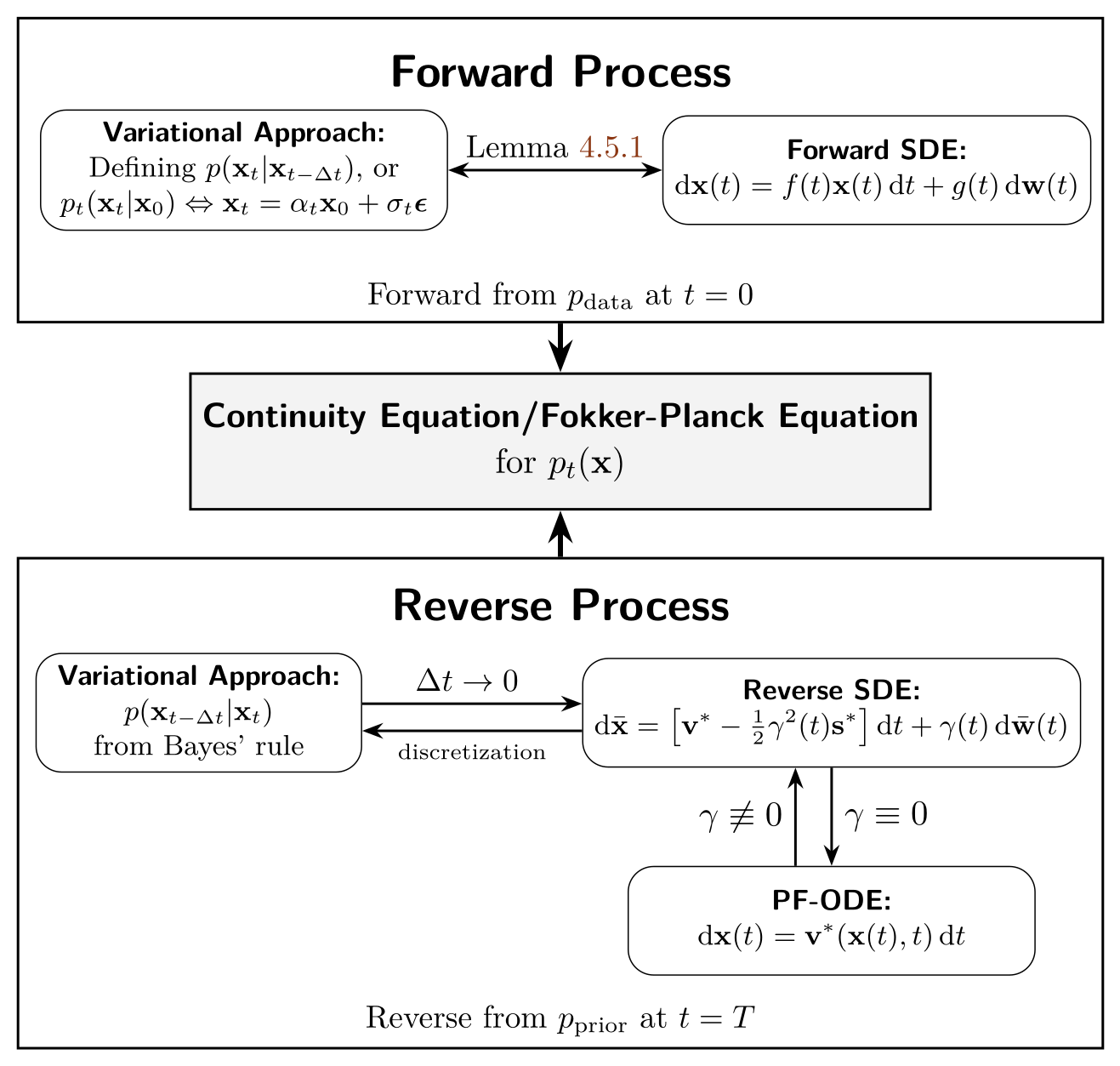
In this section, we show that the three main perspectives of diffusion models—variational, score-based, and flow-based—are not separate constructions but arise from a single unifying principle: the continuity (Fokker–Planck) equation that governs density evolution under a chosen forward process.
First, we recall that the analysis in Section ((Optional) Fokker–Planck Equation and Reverse-Time SDEs : via Marginalization and Bayes’ Rule) in Chapter 4 unifies the variational perspective, based on discrete kernels and Bayes’ rule, with the score-based SDE perspective of continuous dynamics. We establish this connection by showing that variational models act as consistent discretizations of the underlying forward and reverse SDEs. Specifically, the marginal densities calculated step-by-step via the discrete kernels evolve in a manner consistent with the Fokker–Planck equation that governs the continuous-time dynamics. This confirms that the two perspectives are fundamentally equivalent.
We then connect the flow-based and score-based views. In Section 1.4.1, we show that an ODE flow determines a density path whose marginals can always be realized by a family of stochastic processes. This places deterministic flows and stochastic SDEs within the same family.
Together, these results unify the three perspectives under one framework (see Figure 1.2). At last, we conclude this chapter in Section 1.5.
Connection of Flow-Based Approach and Score SDE
A remarkable aspect of diffusion model lies in how different dynamic systems, deterministic or stochastic, can trace out the same evolution of probability distributions. In this section, we reveal a natural and elegant connection between ODE-based flows of Section (Flow Matching FrameworkFlow Matching Framework) in Chapter 5 and Score SDEs. Specifically, we show that the velocity field defining a generative ODE can be transformed into a stochastic counterpart that follows the same Fokker-Planck dynamics, providing a principled bridge between deterministic interpolation and stochastic sampling. This offers us a continuous family of models, ranging from ODEs to SDEs, that generate the same data distribution path.
We consider the continuous-time setup where the perturbation kernel is given by \[p_t({\mathbf{x}}_t|{\mathbf{x}}_0) = \mathcal{N}({\mathbf{x}}_t; \alpha_t {\mathbf{x}}_0, \sigma_t^2 {\mathbf{I}}),\] where \({\mathbf{x}}_0 \sim p_{\mathrm{data}}\). This conditional distribution induces a marginal density path \(p_t({\mathbf{x}}_t) = \mathbb{E}_{{\mathbf{x}}_0 \sim p_{\mathrm{data}}}[p({\mathbf{x}}_t|{\mathbf{x}}_0)]\) as usual, with \(p_T\approx p_{\mathrm{prior}}\).
To match this density path, consider the ODE \[\begin{align} \label{eq:ode-velocity} \frac{\mathop{}\!\mathrm{d}{\mathbf{x}}(t)}{\mathop{}\!\mathrm{d}t} = \mathbf{v}_t({\mathbf{x}}(t)), \quad t \in [0,T], \end{align}\] where \(\mathbf{v}_t({\mathbf{x}}) =\mathbb{E}\left[\alpha_t'{\mathbf{x}}_0+\sigma_t'{\bm{\epsilon}}|{\mathbf{x}}\right]\) is the oracle velocity as shown in Equation in Chapter 5 (noting that time is flipped to follow the diffusion model convention). Integrating \(\eqref{eq:ode-velocity}\) backward from \({\mathbf{x}}(T)\sim p_{\mathrm{prior}}\) yields samples from \(p_0\).
Although this ODE suffices for generating high-quality samples, incorporating stochasticity may improve sample diversity. This motivates the following question:
Is there an SDE whose dynamics, starting from \(p_{\mathrm{prior}}\), yield the same marginal densities as the ODE in Equation \(\eqref{eq:ode-velocity}\)?
This statement affirms that there exists a family of reverse-time SDEs that induce the same marginal density path as the corresponding PF-ODE. The densities induced by these SDEs satisfy the same Fokker–Planck equation for this path, and therefore their one time marginals coincide with the prescribed interpolation \(\{p_t\}_{t\in[0,T]}\)2.
Proposition: Reverse-Time SDEs Generate the Same Marginals as Interpolations
Let \(\gamma(t) \geq 0\) be an arbitrary time-dependent coefficient. Consider the reverse-time SDE, written in the original time variable \(t\) and integrated backward from \(T\) to \(0\), \[\begin{align} \label{eq:general-reverse-sde} \mathop{}\!\mathrm{d}\bar{\mathbf{x}}(t) = \Big[ {\mathbf{v}}^*(\bar{\mathbf{x}}(t), t) - \tfrac{1}{2}\gamma^2(t){\mathbf{s}}^*(\bar{\mathbf{x}}(t), t) \Big]\mathop{}\!\mathrm{d}t + \gamma(t)\mathop{}\!\mathrm{d}\bar{{\mathbf{w}}}(t), \qquad t:T\to 0 . \end{align}\] with terminal condition \(\bar{\mathbf{x}}(T)\sim p_T\). Then this process \(\{\bar{\mathbf{x}}(t)\}_{t\in[0,T]}\) matches the prescribed marginals \(\{p_t\}_{t\in[0,T]}\) induced by the ODE’s density path. Here, \({\mathbf{s}}^*({\mathbf{x}},t):=\nabla_{{\mathbf{x}}}\log p_t({\mathbf{x}})\) is the score function, and it is related to the velocity field \({\mathbf{v}}^*({\mathbf{x}},t)\) by \[\begin{align} \label{eq:score-velocity} {\mathbf{v}}^*({\mathbf{x}}, t) = f(t){\mathbf{x}} - \frac{1}{2}g^2(t){\mathbf{s}}^*({\mathbf{x}},t), \quad {\mathbf{s}}^*({\mathbf{x}},t) = \frac{1}{\sigma_t} \frac{\alpha_t{\mathbf{v}}^*({\mathbf{x}},t)-\alpha_t'{\mathbf{x}}} {\alpha_t'\sigma_t-\alpha_t\sigma_t'} . \end{align}\]
Proof for Proposition. The reverse-time Fokker–Planck equation, written with respect to the original time variable \(t\) while the process is integrated backward, is \[\partial_t p_t = -\nabla\cdot \Big( \big[ {\mathbf{v}}^* - \tfrac{1}{2}\gamma^2{\mathbf{s}}^* \big]p_t \Big) - \tfrac{1}{2}\gamma^2\Delta p_t .\] Using the identity \(\nabla\cdot({\mathbf{s}}^*p_t)=\Delta p_t\) since \({\mathbf{s}}^*=\nabla\log p_t\), the second-order terms cancel, yielding \[\partial_t p_t = -\nabla\cdot({\mathbf{v}}^*p_t),\] i.e., the first-order continuity equation associated with the PF-ODE. Hence the reverse-time SDE and the ODE induce the same marginal density path \(\{p_t\}\). See Appendix A.2–A.3 of Ma et al. (2024). ■
At the oracle level of Proposition: Reverse-Time SDEs Generate the Same Marginals as Interpolations, \(\gamma(t)\) can be chosen arbitrarily without changing the prescribed marginal density path: the \(\gamma\)-dependent drift and diffusion terms cancel exactly in the Fokker–Planck equation. Some representative choices are:
Setting \(\gamma(t) = 0\) recovers the ODE in Equation \(\eqref{eq:ode-velocity}\).
When \(\gamma(t) = g(t)\), Equation \(\eqref{eq:general-reverse-sde}\) becomes the reverse-time SDE in Equation in Chapter 4, since the oracle velocity \({\mathbf{v}}({\mathbf{x}}, t)\) satisfies (see Proposition: Equivalence of Parametrizations): \[{\mathbf{v}}^*({\mathbf{x}}, t) = f(t){\mathbf{x}}- \tfrac{1}{2}g^2(t){\mathbf{s}}^*({\mathbf{x}}, t).\]
Other choices for \(\gamma(t)\) have been explored; e.g., Ma et al. (2024) select \(\gamma(t)\) to minimize the KL gap between \(p_{\mathrm{data}}\) and the \(t=0\) density obtained by solving Equation \(\eqref{eq:general-reverse-sde}\) from \(t=T\).
Following Score SDE, the trained velocity field \({\mathbf{v}}_{\bm{\phi}^\times}({\mathbf{x}}, t)\) can be converted into a parameterized score function \({\mathbf{s}}_{\bm{\phi}^\times}({\mathbf{x}}, t)\) via Equation \(\eqref{eq:score-velocity}\). Plugging this into Equation \(\eqref{eq:general-reverse-sde}\) defines an empirical reverse-time SDE, which can be sampled by numerically integrating from \(t=T\) with \(\bar{\mathbf{x}}(T) \sim p_{\mathrm{prior}}\).
This proposition highlights a remarkable flexibility of diffusion models: once a marginal density path \(\{p_t\}_{t\in[0,T]}\) is induced by the forward process, it can be realized by an entire family of reverse-time dynamics, including the PF-ODE and the reverse-time SDEs \[\mathop{}\!\mathrm{d}\bar{\mathbf{x}}(t) = \big[ {\mathbf{v}}^*(\bar{\mathbf{x}},t) -\tfrac12\gamma^2(t){\mathbf{s}}^*(\bar{\mathbf{x}},t) \big]\mathop{}\!\mathrm{d}t + \gamma(t)\mathop{}\!\mathrm{d}\bar{\mathbf{w}}(t), \quad \gamma(t)\geq0,\] from \(t=T\) to \(t=0\). Although \(\gamma(t)\) changes the stochastic dynamics of individual trajectories, the corresponding Fokker–Planck equations all reduce, for the prescribed density path, to the same governing density equation: \[\partial_t p_t = -\nabla_{{\mathbf{x}}}\cdot \bigl({\mathbf{v}}^*({\mathbf{x}},t)p_t({\mathbf{x}})\bigr).\] Indeed, using \({\mathbf{s}}^*({\mathbf{x}},t)=\nabla_{{\mathbf{x}}}\log p_t({\mathbf{x}})\), the additional \(\gamma\)-dependent drift and diffusion terms cancel at the density level. Thus, \(\gamma(t)\) controls the stochasticity of sample trajectories while preserving the same oracle one-time marginals, connecting the deterministic PF-ODE with a family of stochastic SDE counterparts, as illustrated in Figure 1.2.
Closing Remarks
This chapter has served as the keystone of our theoretical exploration, synthesizing the variational, score-based, and flow-based perspectives into a single, cohesive framework. We have shown that these three seemingly distinct approaches are not merely parallel but are deeply and fundamentally interconnected.
Our unification rests on two core insights. First, we identified the secret sauce common to all frameworks: a conditioning trick that transforms an intractable marginal training objective into a tractable conditional one, enabling stable and efficient learning. Second, we established that the Fokker-Planck equation is the universal law governing the evolution of probability densities. All three perspectives, in their own way, construct a generative process that respects this fundamental dynamic.
Furthermore, we showed that the oracle noise, clean-data, score, and velocity predictions contain the same information and can be converted into one another algebraically. This oracle equivalence does not make the prediction parameterization merely cosmetic: finite-capacity networks may approximate these targets differently, their training objectives can weight errors across noise levels differently, and finite-step numerical solvers can behave differently depending on the representation in which the dynamics are approximated. The important lesson is therefore to distinguish equivalence of the underlying continuous theory from equivalence of a practical training or sampling algorithm. At the density level, however, the common principle remains: modern diffusion methods construct dynamics whose marginals transport a simple prior toward the data distribution along a prescribed probability path.
With this unified and principled foundation firmly established, we are now equipped to move from the foundational theory to the practical application and acceleration of diffusion models. The central insight that generation is equivalent to solving a differential equation provides a powerful platform for control and optimization. The subsequent parts of this monograph will leverage this unified understanding to address key practical challenges:
Part C will focus on improving the sampling process at inference time. We will explore how to steer the generative trajectory for controllable generation (Chapter 8) and investigate advanced numerical solvers to dramatically accelerate the slow, iterative sampling process (Chapter 9).
Part D will then look beyond iterative solvers to learn fast generators directly. We will examine methods that can produce high-quality samples in just one or a few steps, either through distillation from a teacher model (Chapter 10) or by training from scratch (Chapter 11).
Having unified the what and why of diffusion models, we now turn our attention to the exciting and practical frontiers of how.
To see why monotonicity matters, define the remaining variational cost from noise level \(t\) onward as \[L(t;{\mathbf{x}}_0) := \mathcal{D}_{\mathrm{KL}} \left( p({\mathbf{x}}_{[t,T]}|{\mathbf{x}}_0) \,\Vert\, p_{\bm{\phi}}({\mathbf{x}}_{[t,T]}) \right),\] where \({\mathbf{x}}_{[t,T]}:=\{{\mathbf{x}}_s\}_{s\in[t,T]}\) denotes the remaining continuous diffusion path. This is the continuous-time counterpart of the negative ELBO in Equation in Chapter 2, starting from corruption level \(t\); more precisely, it equals the expected negative ELBO of the perturbed sample \({\mathbf{x}}_t\), up to terms independent of \(\bm{\phi}\).
For \({\bm{\epsilon}}\)-prediction, Kingma and Gao (2023) show that \[\frac{\mathop{}\!\mathrm{d}}{\mathop{}\!\mathrm{d}t}L(t;{\mathbf{x}}_0) = \frac{1}{2}\frac{\mathop{}\!\mathrm{d}\Lambda_t}{\mathop{}\!\mathrm{d}t} \mathbb{E}_{{\bm{\epsilon}}} \left[ \left\| {\bm{\epsilon}}_{\bm{\phi}}({\mathbf{x}}_t,t)-{\bm{\epsilon}} \right\|_2^2 \right].\] Hence the weighted diffusion loss is \[-\int_0^T w(\Lambda_t) \frac{\mathop{}\!\mathrm{d}}{\mathop{}\!\mathrm{d}t}L(t;{\mathbf{x}}_0)\mathop{}\!\mathrm{d}t = w(\Lambda_0)L(0;{\mathbf{x}}_0) + \int_0^T \frac{\mathop{}\!\mathrm{d}}{\mathop{}\!\mathrm{d}t}w(\Lambda_t) L(t;{\mathbf{x}}_0)\mathop{}\!\mathrm{d}t + C,\] where \(C\) is independent of \(\bm{\phi}\). If \(w(\Lambda)\) is non-increasing in \(\Lambda\), then \(\frac{\mathop{}\!\mathrm{d}}{\mathop{}\!\mathrm{d}t}w(\Lambda_t)\geq0\) because \(\Lambda_t\) decreases with \(t\). Thus, after normalization, the terms above form a nonnegative weighting over ELBOs at different Gaussian corruption levels, which gives the ELBO-with-Gaussian-augmentation interpretation.↩︎
For completeness, a forward SDE representation (not needed here) is \[\mathop{}\!\mathrm{d}{\mathbf{x}}(t)=f(t) {\mathbf{x}}(t) \mathop{}\!\mathrm{d}t+g(t) \mathop{}\!\mathrm{d}{\mathbf{w}}(t),\] with \(f(t)\) and \(g(t)\) related to \((\alpha_t,\sigma_t)\) via Equation in Chapter 4.↩︎