Chapter 4: Diffusion Models Today: Score SDE Framework
There is only one precise way of presenting the laws, and that is by means of differential equations. They have the advantage of being fundamental and, so far as we know, precise.
Richard P. Feynman
So far, we have studied diffusion models from two perspectives: the variational view and the score-based view, the latter naturally emerging from the EBM formulation. We now take the next step and move to the continuous-time framework. At its core lies the Score SDE (Song et al. 2020), which provides a continuous-time view that brings DDPM and NCSN under the same framework.
Instead of working with only a finite sequence of noise levels, we imagine inserting more and more intermediate levels between data and noise. In the continuous-time limit, the noise level varies smoothly with time, giving the basic picture \[p_{\mathrm{data}} \;\xrightarrow{\text{forward SDE}}\; p_T \approx p_{\mathrm{prior}}, \qquad p_{\mathrm{prior}} \;\xrightarrow{\text{reverse dynamics}}\; p_{\mathrm{data}}.\] The forward SDE describes how data is gradually corrupted into noise, playing the continuous-time role of the noise schedule in DDPM or the sequence of noise levels in NCSN. Once this forward process is specified, the main challenge is generation in the opposite direction: starting from a simple noise distribution, how can we recover the data distribution?
The key quantity is the time-dependent score \[\nabla_{{\mathbf{x}}}\log p_t({\mathbf{x}}),\] which describes the local geometry of the noisy distribution at every time \(t\). Once this score is known, or approximated by a neural network, it determines the reverse-time dynamics used for generation, transforming noise into data. This leads to two complementary descriptions: a stochastic reverse-time SDE and a deterministic probability flow ODE (PF-ODE). Although their sample trajectories are different, they can follow the same evolution of marginal distributions.
This continuous-time view turns generation into the problem of solving differential equations, opening the door to a broad set of tools from stochastic processes, differential equations, and numerical analysis. In particular, once the generative dynamics are written as an SDE or ODE, standard numerical methods can be used to simulate them, while more advanced solvers can improve sampling efficiency and accuracy. This perspective therefore provides not only a unified mathematical description of diffusion models, but also a practical foundation for understanding and designing faster sampling methods developed later in this book.
After this chapter, you will be able to...
understand how the discrete noise levels of DDPM and NCSN lead to a continuous-time forward SDE that gradually transforms data into noise;
understand how generation from noise back to data can be described either by a stochastic reverse-time SDE or by a deterministic probability flow ODE (PF-ODE);
explain how the reverse-time SDE and PF-ODE can follow the same sequence of marginal distributions even though their individual sample trajectories are different, and understand how the Fokker–Planck equation describes the continuous-time evolution of probability densities;
understand how the time-dependent score is learned by denoising score matching and then used for sampling through the reverse-time SDE or PF-ODE;
understand how the PF-ODE can also be run forward for inversion and track changes in probability density through the continuous change-of-variables formula, enabling likelihood evaluation;
recognize VE and VP SDEs as two important instances of the same continuous-time diffusion framework, connecting back to NCSN and DDPM.
Reader route. Readers new to stochastic differential equations may consult the differential-equation appendices in Appendix A as needed. For a first pass, focus on the roles of the forward SDE, reverse-time SDE, and PF-ODE, together with their training and sampling procedures. The Gaussian example and optional derivations can be revisited after the main picture is clear.
Score SDE: Its Principles
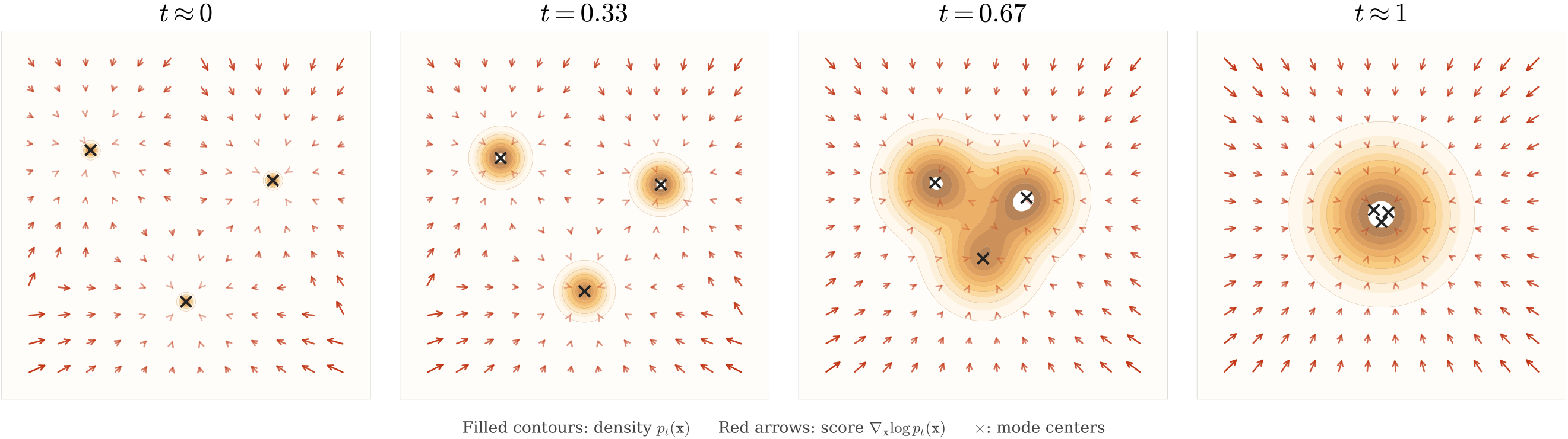
The use of multiple noise scales has been a crucial ingredient in the success of NCSN and DDPM frameworks. In this section, we introduce the foundation of the Score SDE (Song et al. 2020), which elevates this idea by considering a continuum of noise levels. A continuous-time limit of forward and reverse diffusion processes had already been noted by Sohl-Dickstein et al. (2015), but Song et al. (2020) make this perspective central by formulating the data evolution as a stochastic/ordinary differential equation, where the noise level increases smoothly over time. Central to this formulation is the time-dependent score function \(\nabla_{{\mathbf{x}}}\log p_t({\mathbf{x}})\): at each noise level \(t\), it points toward regions of higher density under the current noisy distribution \(p_t\), and it is precisely this quantity that determines how to reverse the diffusion. As Figure 1.1 illustrates, the score field evolves from sharply converging toward individual data modes at small \(t\) to pointing gently toward the global center at large \(t\). This continuous-time formulation not only unifies prior discrete-time models but also provides a principled and flexible foundation for generative modeling: learning this family of score functions across all noise levels reduces generation to the problem of solving differential equations.
Motivation: From Discrete to Continuous-Time Processes
We revisit the forward noise injection schemes of NCSN and DDPM. NCSN uses a sequence of increasing noise levels \(\{\sigma_i\}_{i=1}^L\). Each clean sample \({\mathbf{x}}_0 \sim p_{\mathrm{data}}\) is perturbed as \[{\mathbf{x}}_{\sigma_i} = {\mathbf{x}}_0 + \sigma_i \bm{\epsilon}_i, \qquad \bm{\epsilon}_i \sim \mathcal{N}(\bm{0}, {\mathbf{I}}).\] DDPM instead injects noise incrementally with a variance schedule \(\{\beta_i\}_{i=1}^L\)1: \[{\mathbf{x}}_i = \sqrt{1 - \beta_i}\, {\mathbf{x}}_{i-1} + \sqrt{\beta_i}\, \bm{\epsilon}_i, \qquad \bm{\epsilon}_i \sim \mathcal{N}(\bm{0}, {\mathbf{I}}).\]
We view them together on a discrete time grid, where the sequential update from \({\mathbf{x}}_t\) to \({\mathbf{x}}_{t+\Delta t}\) takes the form2: \[\begin{align*} \mathbf{NCSN:} \,\, & {\mathbf{x}}_{t+\Delta t} = {\mathbf{x}}_t + \sqrt{\sigma_{t+\Delta t}^2 - \sigma_t^2} \bm{\epsilon}_t &&\approx {\mathbf{x}}_t + \sqrt{\frac{\mathop{}\!\mathrm{d}\sigma_t^2}{\mathop{}\!\mathrm{d}t} \Delta t} \bm{\epsilon}_t \\[0.5em] \mathbf{DDPM:} \,\, & {\mathbf{x}}_{t+\Delta t} = \sqrt{1 - \beta(t)\Delta t} {\mathbf{x}}_t + \sqrt{\beta(t)\Delta t} \bm{\epsilon}_t &&\approx {\mathbf{x}}_t - \frac{1}{2} \beta(t) {\mathbf{x}}_t \Delta t + \sqrt{\beta(t)\Delta t} \bm{\epsilon}_t, \end{align*}\] where \(\bm{\epsilon}_t \sim \mathcal{N}(\bm{0}, {\mathbf{I}})\). Interestingly, both noise injection processes follow a common structural pattern: \[\begin{align} \label{eq:euler-discrete-sde} {\mathbf{x}}_{t+\Delta t} \approx {\mathbf{x}}_t + {\mathbf{f}}({\mathbf{x}}_t, t) \Delta t + g(t) \sqrt{\Delta t}\, \bm{\epsilon}_t, \end{align}\] with \({\mathbf{f}}: \mathbb{R}^D \times \mathbb{R} \to \mathbb{R}^D\) and \(g: \mathbb{R} \to \mathbb{R}\) given by: \[\begin{align*} \mathbf{NCSN:} \quad & {\mathbf{f}}({\mathbf{x}}, t) = 0, \qquad g(t) = \sqrt{\frac{\mathop{}\!\mathrm{d}\sigma^2(t)}{\mathop{}\!\mathrm{d}t}} \\[0.5em] \mathbf{DDPM:} \quad & {\mathbf{f}}({\mathbf{x}}, t) = -\frac{1}{2} \beta(t)\, {\mathbf{x}}, \qquad g(t) = \sqrt{\beta(t)}. \end{align*}\]
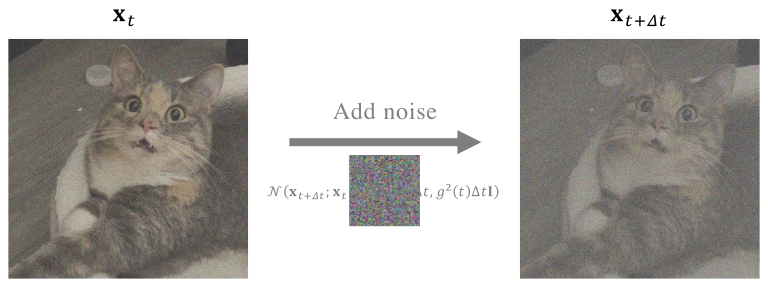
This formulation corresponds to the following Gaussian transition: \[\begin{align} \label{eq:transition-forward-f-g} p({\mathbf{x}}_{t+\Delta t} |{\mathbf{x}}_t) := \mathcal{N}\!\left({\mathbf{x}}_{t+\Delta t}; {\mathbf{x}}_t + {\mathbf{f}}({\mathbf{x}}_t, t)\Delta t,\, g^2(t)\Delta t\, {\mathbf{I}}\right), \end{align}\] where, by a slight abuse of notation, we treat \({\mathbf{x}}_t\) as a fixed sample and \({\mathbf{x}}_{t+\Delta t}\) as a random variable.
As \(\Delta t \to 0\) (which can be conceptually understood as preparing infinitely many layers of noises), the discrete-time process converges to a continuous time SDE evolving forward in time3: \[\begin{align*} \mathop{}\!\mathrm{d}{\mathbf{x}}(t) = {\mathbf{f}}({\mathbf{x}}(t), t) \mathop{}\!\mathrm{d}t + g(t) \mathop{}\!\mathrm{d}{\mathbf{w}}(t), \end{align*}\] where \({\mathbf{w}}(t)\) is a standard Wiener process (or Brownian motion).
Remark. While a full formal definition is not necessary here, a Wiener process is a continuous-time stochastic process \({\mathbf{w}}(t)\) that starts at zero, has independent increments, and satisfies that for any \(s < t\), the increment \({\mathbf{w}}(t) - {\mathbf{w}}(s)\) is normally distributed with mean zero and variance \(t - s\). It represents the accumulation of independent Gaussian fluctuations over time, and although it is almost surely continuous, it is nowhere differentiable.
Over an infinitesimal time interval \([t, t + \mathop{}\!\mathrm{d}t]\), the increment of a Wiener process is defined as \[\mathop{}\!\mathrm{d}{\mathbf{w}}(t) := {\mathbf{w}}(t + \mathop{}\!\mathrm{d}t) - {\mathbf{w}}(t),\] which is modeled as a Gaussian random variable with zero mean and variance \(\mathop{}\!\mathrm{d}t\): \[\mathop{}\!\mathrm{d}{\mathbf{w}}(t) \sim \mathcal{N}(\bm{0}, \mathop{}\!\mathrm{d}t {\mathbf{I}}).\]
A brief introduction to the foundations of SDEs is provided in Appendix C, with a more advanced discussion in Appendix C. However, we can conceptually understand the connection between the discrete and continuous formulations as follows:
\({\mathbf{x}}(t+\Delta t) - {\mathbf{x}}(t) \approx \mathop{}\!\mathrm{d}{\mathbf{x}}(t)\),
\(\Delta t \approx \mathop{}\!\mathrm{d}t\),
\(\sqrt{\Delta t} \bm{\epsilon}_t \sim \mathcal{N}(\bm{0}, \Delta t {\mathbf{I}}) \approx \mathop{}\!\mathrm{d}{\mathbf{w}}(t)\).
Once the drift \({\mathbf{f}}({\mathbf{x}},t)\) and diffusion \(g(t)\) are specified, the forward time SDE automatically induces a reverse time SDE that transports the terminal noise distribution back to the data distribution. The reverse dynamics involve only a single unknown term, surprisingly the score function at each continuous-time level. This identifies score matching as the training objective; once the score is learned, sampling amounts to numerically integrating the reverse time SDE with the learned score.
While Section 1.3 presents practical implementations, we first examine the theoretical foundations of the forward and reverse processes in Section 1.1.2 and Section 1.1.3.
Forward-Time SDEs: From Data to Noise
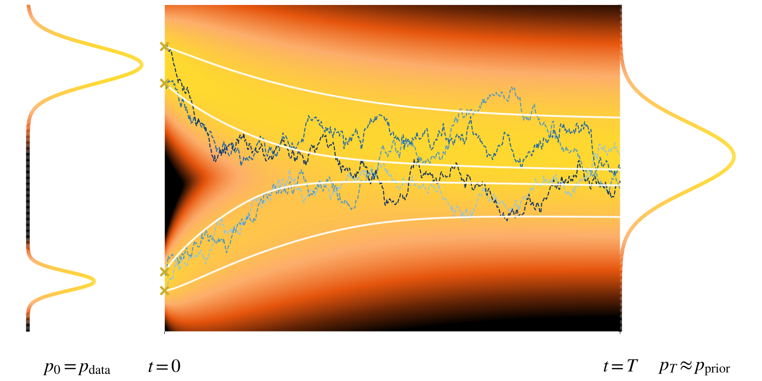
With this formulation, earlier methods based on discrete time, such as NCSN (Song and Ermon 2019) and DDPM (Sohl-Dickstein et al. 2015; Ho et al. 2020), can be unified under the continuous-time framework through a stochastic process \({\mathbf{x}}(t)\) governed by a forward SDE defined on the interval \([0, T]\):
\[\begin{equation} \label{eq:sde_forward} \mathop{}\!\mathrm{d}{\mathbf{x}}(t) = \mathbf{f}({\mathbf{x}}(t), t) \mathop{}\!\mathrm{d}t + g(t) \mathop{}\!\mathrm{d}{\mathbf{w}}(t), \quad {\mathbf{x}}(0) \sim p_{\mathrm{data}}. \end{equation}\]
Here, \(\mathbf{f}(\cdot, t)\colon\mathbb{R}^D\to\mathbb{R}^D\) is the drift, \(g(t) \in \mathbb{R}\) is the scalar diffusion coefficient, and \({\mathbf{w}}(t)\) denotes a standard Wiener process. We refer to this as the forward SDE, which describes how clean data is gradually perturbed into noise over time.
Once the drift \(\mathbf{f}\) and diffusion coefficient \(g\) are specified, the forward process is fully determined, describing how the data variable is progressively corrupted through the injection of Gaussian noise. In particular, two families of time-dependent densities are induced:
Perturbation Kernels.
The conditional law \[p_t({\mathbf{x}}_t |{\mathbf{x}}_0)\] describes how a clean data sample \({\mathbf{x}}_0 \sim p_{\mathrm{data}}\) evolves into its noisy counterpart \({\mathbf{x}}_t\) at time \(t\). In general, the drift term \({\mathbf{f}}({\mathbf{x}},t)\) in Equation \(\eqref{eq:sde_forward}\) can be an arbitrary function of \({\mathbf{x}}\), but a common and analytically convenient choice is to assume it is affine: \[\begin{equation} \label{eq:affine-drift} {\mathbf{f}}({\mathbf{x}},t) = f(t) {\mathbf{x}}, \end{equation}\] where \(f(t)\) is a scalar function of \(t\), typically taken to be non-positive. Under this structure, the conditional process remains Gaussian given \({\mathbf{x}}_0\), and the perturbation kernel admits a closed-form solution obtained by solving the associated mean–variance ODEs (Särkkä and Solin 2019) (see also Section 1.4.3). In particular, \[p_t({\mathbf{x}}_t |{\mathbf{x}}_0) = \mathcal{N} \big({\mathbf{x}}_t; {\mathbf{m}}(t), P(t)\mathbf I_D\big),\] with \[{\mathbf{m}}(t) = \exp \Big(\int_0^t f(u) \mathop{}\!\mathrm{d}u\Big) {\mathbf{x}}_0, \quad P(t) = \int_0^t \exp \Big(2 \int_s^t f(u) \mathop{}\!\mathrm{d}u\Big) g^2(s) \mathop{}\!\mathrm{d}s,\] and initial conditions \({\mathbf{m}}(0)={\mathbf{x}}_0\), \(P(0)=0\).
This explicit form allows one to sample \({\mathbf{x}}_t\) given \({\mathbf{x}}_0\) directly, without numerically integrating the SDE, hence the term simulation-free. Both NCSN and DDPM fall into this affine-drift setting.
In the remainder, we develop the general theory for arbitrary drifts \({\mathbf{f}}({\mathbf{x}},t)\), but will return to the affine drift when closed-form analysis is useful.
Marginal Densities.
The time-marginal density \(p_t({\mathbf{x}}_t)\) is obtained by integrating over the perturbation kernel: \[\begin{equation} \label{eq:scoresde-oracle-marginal} p_t({\mathbf{x}}_t) := \int p_t({\mathbf{x}}_t|{\mathbf{x}}_0) p_{\mathrm{data}}({\mathbf{x}}_0) \mathop{}\!\mathrm{d}{\mathbf{x}}_0, \quad \text{with } p_0 = p_{\mathrm{data}}. \end{equation}\]
By choosing the coefficients \(f(t)\) and \(g(t)\) appropriately, the forward process gradually adds noise until the influence of the initial state is effectively forgotten. As \(T\) becomes large, the conditional distribution \(p_T(\mathbf{x}_T |\mathbf{x}_0)\) no longer depends on \(\mathbf{x}_0\), because its mean evolves as \[{\mathbf{m}}(T) = \exp\!\Big(\int_0^T f(u)\mathop{}\!\mathrm{d}u\Big) \mathbf{x}_0 \longrightarrow \mathbf{0}, \quad \text{as } T\to\infty,\] provided \(f(u)\) is non-positive so that the exponential factor decays. At the same time, the variance grows and stabilizes to match a chosen prior distribution. Consequently, the marginal \[p_T(\mathbf{x}_T) = \int p_T(\mathbf{x}_T |\mathbf{x}_0) p_{\mathrm{data}}(\mathbf{x}_0)\mathop{}\!\mathrm{d}\mathbf{x}_0,\] which initially represents a complicated mixture over data samples, converges to a simple prior \(p_{\mathrm{prior}}\), typically Gaussian. In this limit, \[p_T(\mathbf{x}_T) \approx p_{\mathrm{prior}}(\mathbf{x}_T) \quad \text{and} \quad p_T(\mathbf{x}_T |\mathbf{x}_0) \approx p_{\mathrm{prior}}(\mathbf{x}_T),\] so the forward process maps any data distribution into a tractable prior, providing a convenient starting point for reversal and generation.
Reverse-Time Stochastic Process for Generation
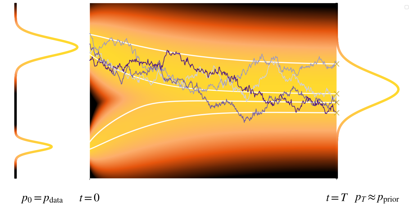
Intuitively, data generation from noise can be achieved by “reversing” the forward process: starting from a random point sampled from the prior distribution and evolving it backward in time to obtain a generated sample. For deterministic systems (that is, ODEs), this idea works naturally. Since no randomness is involved, reversing time simply means tracing the trajectory of a point in the opposite direction along the same path as in the forward process4. In contrast, SDEs incorporate stochasticity at every time step, meaning that a single point can evolve along many plausible random trajectories. As a result, reversing such processes is more subtle5.
While individual stochastic trajectories are not reversible, the remarkable insight is that the distribution over these trajectories can be reversed. This is formalized by a foundational result from Anderson (1982), which shows that the time-reversed process \(\{ \bar{{\mathbf{x}}}(t) \}_{t \in [0, T]}\)6 of the forward process in Equation \(\eqref{eq:sde_forward}\) is itself governed by a well-defined SDE. This reverse-time process evolves from \(T\) to \(0\), and its dynamics are given by:
\[\begin{align} \label{eq:sde_backward} \begin{aligned}[t] \mathop{}\!\mathrm{d}\bar{{\mathbf{x}}}(t) = \left[\mathbf{f}(\bar{{\mathbf{x}}}(t), t) {\color{orange} - g^2(t) \nabla_{{\mathbf{x}}} \log p_t(\bar{{\mathbf{x}}}(t))} \right] \mathop{}\!\mathrm{d}t + g(t) \mathop{}\!\mathrm{d}\bar{{\mathbf{w}}}(t), \\ \quad \bar{{\mathbf{x}}}(T) \sim p_{\mathrm{prior}} \approx p_T. \end{aligned} \end{align}\]
Here, \(\bar{{\mathbf{w}}}(t)\) denotes a standard Wiener process in reverse time, defined as \(\bar{{\mathbf{w}}}(t) := {\mathbf{w}}(T - t) - {\mathbf{w}}(T)\).
Remark. Throughout this chapter, \(t\) denotes the original diffusion clock: \(t=0\) corresponds to data and \(t=T\) to noise. Accordingly, the reverse-time SDE in Equation \(\eqref{eq:sde_backward}\) is integrated from \(t=T\) down to \(t=0\), so \(\mathop{}\!\mathrm{d}t<0\) along the reverse process. Equivalently, one may introduce a forward-running reverse clock \(s:=T-t\); unless stated otherwise, we keep the original clock \(t\).
To build intuition for Equation \(\eqref{eq:sde_backward}\), we present a concrete example in Section 1.2.2 with a Gaussian data distribution and linear–Gaussian dynamics. This setting is analytically tractable: one can derive the time-reversal formula directly using basic calculus and linear algebra, without invoking the full general theory of Anderson (1982).
Note that the presence of stochasticity (\(g\neq 0\)) introduces an additional correction term, \(-g^2(t) \nabla_{{\mathbf{x}}} \log p_t(\bar{{\mathbf{x}}}(t))\), which accounts for the effect of diffusion and ensures that the reversed dynamics correctly reproduce the evolution of marginal distributions induced by the forward SDE (see Section 1.2).
Conceptually, Why Does the Reverse Process Work?
Section 1.6.2 presents an intuitive derivation of the reverse-time SDE by connecting it to the DDPM variational framework (optional but insightful). Here, we provide complementary intuition for how the reverse-time dynamics recover structured data from noise.
At first glance, the presence of Brownian noise in the reverse time process may seem paradoxical. If the forward diffusion spreads data into increasingly noisy configurations, it is unclear how reversing this process, particularly one that introduces additional randomness through \(\bar{{\mathbf{w}}}(t)\), can produce clean, structured samples concentrated near the data manifold. The key point is that the reverse time SDE does not inject arbitrary randomness. The diffusion term \(g(t)\mathop{}\!\mathrm{d}\bar{{\mathbf{w}}}(t)\) is always coupled with the score–driven drift \(- g^2(t)\nabla_{{\mathbf{x}}}\log p_t(\bar{{\mathbf{x}}}(t))\). Together, these terms balance one another: the score guides trajectories toward regions of higher density, while the noise introduces controlled stochasticity that allows exploration without overwhelming the dynamics.
To see this more clearly, return to the Langevin intuition in Equation in Chapter 3. When \(f(t)\equiv 0\), Equation \(\eqref{eq:sde_backward}\) reads \[\mathop{}\!\mathrm{d}\bar{{\mathbf{x}}}(t) = - g^2(t) \nabla_{{\mathbf{x}}}\log p_t\!\big(\bar{{\mathbf{x}}}(t)\big) \mathop{}\!\mathrm{d}t + g(t) \mathop{}\!\mathrm{d}\bar{{\mathbf{w}}}(t).\] Reparameterize time forward via \(s:=T-t\) (so \(\mathop{}\!\mathrm{d}t=-\mathop{}\!\mathrm{d}s\)), and rename the Brownian motion in law so that \(\mathop{}\!\mathrm{d}\bar{{\mathbf{w}}}(t)=-\mathop{}\!\mathrm{d}{\mathbf{w}}_s\). Writing \(\bar{{\mathbf{x}}}_s:=\bar{{\mathbf{x}}}(T-s)\) and \(\pi_s:=p_{T-s}\) then gives \[\begin{align*} \mathop{}\!\mathrm{d}\bar{{\mathbf{x}}}_s &= g^2(T-s) \nabla\log \pi_s \big(\bar{{\mathbf{x}}}_s\big) \mathop{}\!\mathrm{d}s + g(T-s) \mathop{}\!\mathrm{d}{\mathbf{w}}_s \\&= 2\tau(s) \nabla\log \pi_s\!\big(\bar{{\mathbf{x}}}_s\big) \mathop{}\!\mathrm{d}s + \sqrt{2\tau(s)} \mathop{}\!\mathrm{d}{\mathbf{w}}_s, \quad \tau(s):=\tfrac{1}{2}g^2(T-s). \end{align*}\] This has the Langevin form with a time-varying temperature \(\tau(s)\), targeting the evolving density \(\pi_s\). By Tweedie’s formula (Equation in Chapter 3), the score direction \(\nabla\log \pi_s\) points toward the conditional clean signal at each time slice, so the drift continually “pulls back” denoised structure.
Crucially, \(g(t)\) is annealing along the reverse trajectory. Early on (\(s\approx 0\), i.e., \(t\approx T\)), \(g(T-s)\) is typically larger, so the injected noise is stronger and the process explores broadly. As \(s\) increases, \(g(T-s)\) decreases, the stochastic term weakens, and the score term dominates, pulling samples into high-density regions of \(\pi_s\); by \(s=T\) (i.e., \(t=0\)), trajectories concentrate near the data manifold.
Overview of Reverse-Time SDE Capabilities.
It is fascinating how the time-dependent score function \[{\mathbf{s}}({\mathbf{x}}, t) := \nabla_{{\mathbf{x}}} \log p_t({\mathbf{x}})\] naturally appears in Equation \(\eqref{eq:sde_backward}\). Once the forward coefficients \(f(t)\) and \(g(t)\) are specified, the score is the only remaining unknown in the reverse dynamics. This highlights its central role: with the score in hand, the reverse process is determined, and sampling amounts to numerically integrating Equation \(\eqref{eq:sde_backward}\) with the learned score.
Since the oracle score generally lacks a closed-form expression, we adopt the approach of Chapter 3 and train a neural network \(\mathbf{s}_{\bm{\phi}}({\mathbf{x}}, t)\) to approximate it via score matching; see Section 1.3.1 for details. Substituting \({\mathbf{s}}({\mathbf{x}}, t)\) with \(\mathbf{s}_{\bm{\phi}}({\mathbf{x}}, t)\) in Equation \(\eqref{eq:sde_backward}\) then specifies the reverse dynamics completely.
Generation corresponds to solving the reverse-time SDE reversely from \(t = T\), starting with \({\mathbf{x}}_T \sim p_{\mathrm{prior}}\), to \(t = 0\). Importantly, Anderson (1982) proves that the marginal densities of the forward and reverse processes coincide, ensuring that samples at \(t=0\) approximately follow \(p_{\mathrm{data}}\) when \(p_{\mathrm{prior}} \approx p_T\). We will explore this further in Section 1.3.2.
Deterministic Process (Probability Flow ODE) for Generation
Although the SDE in Equation \(\eqref{eq:sde_backward}\) introduces stochasticity and potentially increases the diversity of generated samples, a question arises:
Is it necessary to sample using the SDE in Equation \(\eqref{eq:sde_backward}\)?
Inspired by Maoutsa et al. (2020), Song et al. (2020) also introduced a deterministic process, an ODE, that evolves samples with the same marginal distributions as the forward SDE. This process \(\{\tilde{\mathbf{x}}(t)\}_{t\in[0,T]}\)7, called the Probability Flow ODE (PF-ODE), is given by:
\[\begin{equation} \label{eq:prob_ode_gt} \frac{\mathop{}\!\mathrm{d}}{\mathop{}\!\mathrm{d}t}\tilde{\mathbf{x}}(t) = \mathbf{f}(\tilde{\mathbf{x}}(t), t) - \frac{1}{2} g^2(t) \nabla_{{\mathbf{x}}} \log p_t(\tilde{\mathbf{x}}(t)). \end{equation}\]
Analogous to the SDE case, one can replace the true score with a learned approximation and integrate the reverse-time ODE from \(t = T\) to \(t = 0\) to generate samples. Concretely, the generated sample (solution of PF-ODE at time \(t=0\)) takes the form \[\tilde{\mathbf{x}}(T) + \int_{T}^{0} \Big[ \mathbf{f}(\tilde{\mathbf{x}}(\tau), \tau) - \frac{1}{2} g^2(\tau) \nabla_{{\mathbf{x}}} \log p_\tau(\tilde{\mathbf{x}}(\tau)) \Big] \mathop{}\!\mathrm{d}\tau,\] where the initial condition \(\tilde{\mathbf{x}}(T) \sim p_{\mathrm{prior}}\). Since this integral is intractable in closed form, practical generation relies on numerical solvers (e.g., Euler method, see Equation \(\eqref{eq:euler-maruyama}\)).
Compared to the reverse-time SDE, the PF-ODE offers two key advantages:
The ODE can be integrated in either direction, from \(t=0\) to \(t=T\) or from \(t=T\) to \(t=0\), using the same formulation of the equation, provided the corresponding initial condition is specified at the chosen endpoint. This bidirectionality contrasts with SDEs, which generally admit only forward time integration.
It benefits from a wide range of well-established, off-the-shelf numerical solvers developed for ODEs.
We emphasize that the PF-ODE is not obtained by simply removing the diffusion term in Equation \(\eqref{eq:sde_backward}\); notably, the factor of \(\frac{1}{2}\) in its drift term has a principled origin. At a high level, Equation \(\eqref{eq:prob_ode_gt}\) arises by choosing the drift of an ODE such that its evolution preserves the same marginal densities as the forward SDE in Equation \(\eqref{eq:sde_forward}\). The underlying principle (i.e., Fokker-Planck Equation (Øksendal 2003)) ensuring this alignment of marginals will be detailed in the next section.
Matching Marginals in Forward/Reverse-Time SDEs and PF-ODE
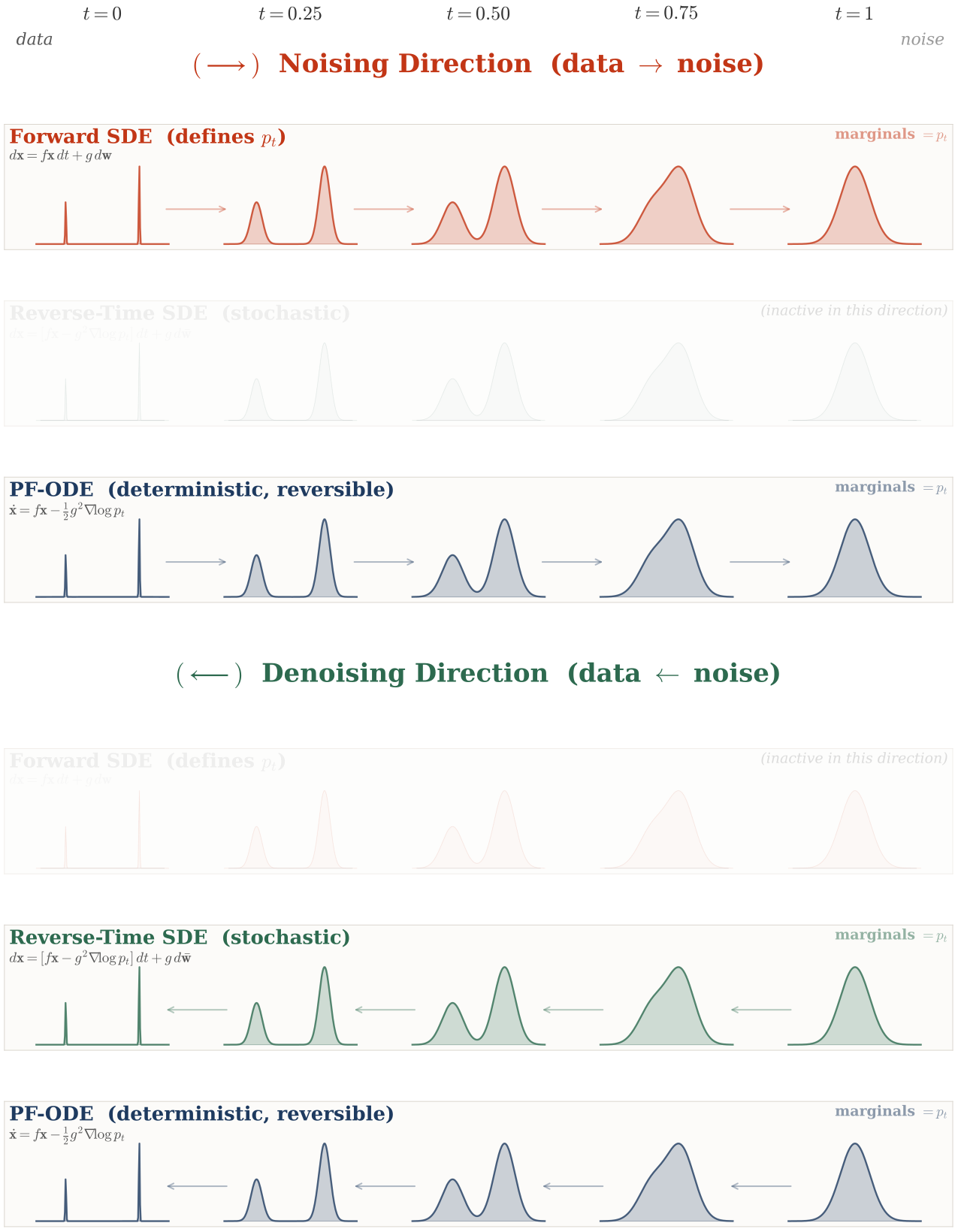
In this section, we present the Fokker-Planck equation as the central principle governing diffusion models. It describes how probability densities evolve under noisy dynamics and serves as the natural analogue of a change-of-variables formula when randomness is present (see Appendix B). Starting from the forward diffusion process, which defines the marginals \(p_t\), we explain how both the reverse-time SDE and the PF-ODE are designed to reproduce the same marginal family. We then make this principle concrete through a Gaussian example, where the reverse-time SDE and the PF-ODE can be computed directly and explicitly.
Fokker-Planck Equation to Ensure Alignment of Marginal Densities
A central concept in diffusion models is that different processes can lead to the same sequence of marginal distributions (as we will illustrate later in this subsection). The objective is to construct a process that transforms \(p_{\mathrm{prior}}\) into \(p_{\mathrm{data}}\) by aligning the marginals across time, and in particular at \(t=0\). The exact form of the process is secondary, provided it is tractable and admits efficient sampling. This naturally leads to a fundamental question:
How can we ensure that different processes yield identical marginal distributions?
Returning to our setup, once the forward SDE is specified, it defines the evolution of marginal densities from \(p_{\mathrm{data}}\) to \(p_{\mathrm{prior}}\). The reverse-time SDE and PF-ODE are then constructed so that their trajectories yield marginal distributions that exactly match those of the forward process. The key to this correspondence lies in the Fokker–Planck equation, which governs how marginal densities evolve under diffusion processes. An illustration is provided in Figure 1.5. The following theorem (Anderson 1982; Song et al. 2020) establishes the foundation for this connection:
Theorem: Marginal Alignment via the Fokker–Planck Equation
Consider the forward SDE \[\mathop{}\!\mathrm{d}{\mathbf{x}}(t) = {\mathbf{f}}({\mathbf{x}}(t),t)\mathop{}\!\mathrm{d}t + g(t)\mathop{}\!\mathrm{d}{\mathbf{w}}(t), \qquad {\mathbf{x}}(0)\sim p_0=p_{\mathrm{data}}.\] Under standard regularity conditions, its marginal density \(p_t\) evolves according to the Fokker–Planck equation \[\begin{align} \label{eq:fp_general} \begin{aligned} \partial_t p_t({\mathbf{x}}) &= -\nabla_{{\mathbf{x}}}\cdot \bigl[{\mathbf{f}}({\mathbf{x}},t)p_t({\mathbf{x}})\bigr] + \tfrac 12 g^2(t)\Delta_{{\mathbf{x}}}p_t({\mathbf{x}}) \\ &= -\nabla_{{\mathbf{x}}}\cdot \bigl[{\mathbf{v}}({\mathbf{x}},t)p_t({\mathbf{x}})\bigr], \end{aligned} \end{align}\] where \(\Delta_{{\mathbf{x}}}\) denotes the Laplacian operator and \[{\mathbf{v}}({\mathbf{x}},t) := {\mathbf{f}}({\mathbf{x}},t) - \tfrac 12 g^2(t) \nabla_{{\mathbf{x}}}\log p_t({\mathbf{x}}).\]
Importantly, the same family of marginal distributions \(\{p_t\}_{t\in[0,T]}\) can be realized by two different dynamics:
The PF-ODE \[\frac{\mathop{}\!\mathrm{d}\tilde{\mathbf{x}}(t)}{\mathop{}\!\mathrm{d}t} = {\mathbf{v}}(\tilde{\mathbf{x}}(t),t).\] Starting from \(\tilde{\mathbf{x}}(0)\sim p_0\) and solving forward from \(0\) to \(T\) gives \(\tilde{\mathbf{x}}(t)\sim p_t\). Equivalently, starting from \(\tilde{\mathbf{x}}(T)\sim p_T\) and solving the same ODE backward from \(T\) to \(0\) follows the same marginals in reverse.
The reverse-time SDE \[\mathop{}\!\mathrm{d}\bar{\mathbf{x}}(t) = \Bigl[ {\mathbf{f}}(\bar{\mathbf{x}}(t),t) - g^2(t)\nabla_{{\mathbf{x}}}\log p_t(\bar{\mathbf{x}}(t)) \Bigr]\mathop{}\!\mathrm{d}t + g(t)\mathop{}\!\mathrm{d}\bar{\mathbf{w}}(t).\] Starting from \(\bar{\mathbf{x}}(T)\sim p_T\), this SDE is solved backward in time from \(t=T\) to \(t=0\). Along this reverse evolution, its marginal distribution at time \(t\) is \[\bar{\mathbf{x}}(t)\sim p_t.\]
Thus, the reverse-time SDE and PF-ODE can have the same marginal distribution at every noise level even though one is stochastic and the other is deterministic.
Proof for Theorem. The proof is provided in Section (Marginal Alignment via Fokker–Planck) in Appendix D, while Section 1.6.1 offers further intuition behind the Fokker–Planck equation using the marginalization technique of probability. ■
Multiple Conditional Distributions for a Fixed Marginal.
To understand how the PF-ODE transports \(p_{\mathrm{data}}\) forward in time (or equivalently \(p_{\mathrm{prior}}\) in reverse), consider the flow map \({\bm{\Psi}}_{s \to t}: \mathbb{R}^D \to \mathbb{R}^D\), where \({\bm{\Psi}}_{s \to t}({\mathbf{x}}_s)\) denotes the PF-ODE solution at time \(t\) initialized from \({\mathbf{x}}_s\) at time \(s\), for any time \(s, t \in[0,T]\). In other words, this map takes an initial state \({\mathbf{x}}_s\) and directly jumps to its state at \(t\): \[\begin{align} \label{eq:flow-map-def} {\bm{\Psi}}_{s \to t}({\mathbf{x}}_s) \mathrel{:=}{\mathbf{x}}_s + \int_s^t {\mathbf{v}}({\mathbf{x}}_\tau, \tau)\mathrm{d}\tau, \end{align}\] with velocity field \[\begin{align*} {\mathbf{v}}({\mathbf{x}}, \tau) := {\mathbf{f}}({\mathbf{x}}, \tau) - \frac{1}{2} g^2(\tau)\nabla_{{\mathbf{x}}}\log p_\tau({\mathbf{x}}). \end{align*}\] Here, the integral captures the net displacement accumulated along the PF-ODE trajectory. The term flow map is indeed classical in differential equations, dynamical systems, and continuum mechanics: it denotes the map that carries a state from its position at time \(s\) to its position at time \(t\) under the given dynamics. The velocity field \({\mathbf{v}}({\mathbf{x}},t)\) describes the instantaneous motion, whereas the flow map \({\bm{\Psi}}_{s\to t}\) records the accumulated motion over a finite time interval (Arnold 1988; Chorin and Marsden 1993)8. We use the term in this standard mathematical and physical sense throughout the book, particularly when discussing fast diffusion-based generators in Chapter 10 and Chapter 11. Under mild smoothness assumptions on \({\mathbf{v}}\), the flow map \({\bm{\Psi}}_{s \to t}: \mathbb{R}^D \to \mathbb{R}^D\) is a smooth bijection9.
For any \(t\in[0,T]\), the pushforward density is defined as \[p_t^{\mathrm{fwd}}({\mathbf{x}}_t) := \int \delta\bigl({\mathbf{x}}_t - {\bm{\Psi}}_{0 \to t}({\mathbf{x}}_0)\bigr)\, p_{\mathrm{data}}({\mathbf{x}}_0) \,\mathop{}\!\mathrm{d}{\mathbf{x}}_0,\] denoted \(\bm{\Psi}_{0\to t} \sharp p_{\mathrm{data}}\), representing the distribution at time \(t\) under \(\bm{\Psi}_{0\to t}\). Theorem: Marginal Alignment via the Fokker–Planck Equation ensures \(p_t^{\mathrm{fwd}} = p_t\), where \(p_t\) is the marginal density of the forward SDE, equating the deterministic PF-ODE and stochastic kernel: \[p_t({\mathbf{x}}_t) = \int p_t({\mathbf{x}}_t |{\mathbf{x}}_0)\, p_{\mathrm{data}}({\mathbf{x}}_0)\,\mathop{}\!\mathrm{d}{\mathbf{x}}_0 = \int \delta\bigl({\mathbf{x}}_t - \bm{\Psi}_{0\to t}({\mathbf{x}}_0)\bigr)\, p_{\mathrm{data}}({\mathbf{x}}_0)\,\mathop{}\!\mathrm{d}{\mathbf{x}}_0.\]
This implies infinitely many conditionals \(Q_t({\mathbf{x}}_t |{\mathbf{x}}_0)\) yield the same \(p_t({\mathbf{x}}_t)\), for instance:
Stochastic (Simulation-Free): \(Q_t({\mathbf{x}}_t |{\mathbf{x}}_0) = p_t({\mathbf{x}}_t |{\mathbf{x}}_0)\),
Deterministic (Requires ODE Solving): \(Q_t({\mathbf{x}}_t |{\mathbf{x}}_0) = \delta\bigl({\mathbf{x}}_t - \bm{\Psi}_{0\to t}({\mathbf{x}}_0)\bigr)\),
Mixture: \(Q_t({\mathbf{x}}_t |{\mathbf{x}}_0) = \lambda p_t({\mathbf{x}}_t |{\mathbf{x}}_0) + (1-\lambda)\delta\bigl({\mathbf{x}}_t - \bm{\Psi}_{0\to t}({\mathbf{x}}_0)\bigr)\), \(\lambda\in[0,1]\).
This nonuniqueness of \(Q_t({\mathbf{x}}_t |{\mathbf{x}}_0)\) arises from the fact that the marginal constraint does not uniquely determine the conditional distribution. This concept reappears in Section (Flow Matching Framework) in Chapter 5 and Section ((Optional) The Original Variational Perspective on DDIM) in Chapter 9. In particular, there exists an entire family of reverse-time SDEs that are consistent with the same marginal \(p_t\).
Observation: Matching Prescribed Marginal Densities
Multiple processes can give rise to the same sequence of marginal densities; what truly matters is satisfying the Fokker–Planck equation. This fundamental insight affords us remarkable flexibility in designing generative processes that transition from \(p_{\mathrm{prior}}\) to \(p_{\mathrm{data}}\), or vice versa.
The Fokker–Planck equation lies at the heart of diffusion models and is rooted in the fundamental change-of-variable formula for probability densities (see Appendix B for a systematic treatment). Far from being a minor technical detail, this principle recurs throughout our development, most notably in Section (Flow Matching FrameworkFlow Matching Framework) in Chapter 5.
A Computable Example: Evolutions of Gaussian Dynamics
When \(p_{\mathrm{data}}\) is a normal distribution (or a mixture of Gaussians), the score function admits a closed-form expression. This makes it an ideal setting for building intuition about diffusion processes: we can explicitly derive the reverse-time SDE and the PF-ODE using only basic calculus, without resorting to advanced mathematical tools. In this subsection, we illustrate how these equations behave in such a tractable case.
Exact Computation of the Reverse-Time SDE with a Gaussian.
When \(p_{\mathrm{data}}\) is Gaussian, the formula in Equation \(\eqref{eq:sde_backward}\) can be derived directly, without relying on the general theory and proofs of Anderson (1982). To illustrate the core idea, we consider the one-dimensional case; the extension to higher dimensions follows in the same way.
Start from the forward SDE \[\mathop{}\!\mathrm{d}x(t) = f(t) x(t) \mathop{}\!\mathrm{d}t + g(t) \mathop{}\!\mathrm{d}w_t,\] and take one small Euler step of size \(\Delta t>0\): \[x_{t+\Delta t} = a x_t + r \epsilon,\] where \(a:=1+f(t)\Delta t\), \(r:=g(t)\sqrt{\Delta t}\), and \(\epsilon\sim\mathcal N(0,1)\). Equivalently, the forward one-step transition kernel is Gaussian: \[x_{t+\Delta t} | x_t \sim \mathcal N\!\big(\cdot;a x_t, r^2\big).\] Since \(p_{\mathrm{data}}\) is assumed to be Gaussian, the current marginal at time \(t\) is also Gaussian, which takes the following form: \[x_t \sim \mathcal N(\cdot;m_t, s_t^2),\] for some scalar \(m_t\) and \(s_t\). So conditioning will amount to multiplying two Gaussians and renormalizing. This keeps the algebra elementary.
By Bayes’ rule the conditional density is, up to a constant, the product of the prior and the transition kernel: \[\begin{align*} p(x_t | x_{t+\Delta t}) &\propto p(x_{t+\Delta t} | x_t ) p_t({\mathbf{x}}_t) \\&\propto \exp\Big(-\frac{(x_t-m_t)^2}{2s_t^2}\Big) \exp\Big(-\frac{(x_{t+\Delta t}-a x_t)^2}{2r^2}\Big). \end{align*}\] The exponent is a quadratic in \(x_t\). Expanding both squares and grouping terms shows exactly which coefficients matter: \[-2\log p(x_t | x_{t+\Delta t}) = A x_t^2 - 2 B x_t + \text{const},\] with \[A:=\frac{1}{s_t^2}+\frac{a^2}{r^2},\quad B:=\frac{m_t}{s_t^2}+\frac{a x_{t+\Delta t}}{r^2}.\] Here \(A\) is the sum of precisions (prior precision plus the transition-kernel precision transported through \(a\)), while \(B\) is the corresponding precision-weighted sum of targets. With these in hand, completing the square gives the posterior in one line: \[A x_t^2 - 2 B x_t = A\Big(x_t-\frac{B}{A}\Big)^2 - \frac{B^2}{A},\] so the conditional distribution is Gaussian with variance \(1/A\) and mean \(B/A\): \[\mathrm{Var}(x_t | x_{t+\Delta t}) = \frac{1}{\frac{1}{s_t^2}+\frac{a^2}{r^2}}, \qquad \mathbb E[x_t | x_{t+\Delta t}] = \frac{\frac{m_t}{s_t^2}+\frac{a x_{t+\Delta t}}{r^2}}{\frac{1}{s_t^2}+\frac{a^2}{r^2}}.\] These closed forms already describe the reverse transition for any small \(\Delta t\). To read off a reverse-time SDE, we now expand them for small \(\Delta t\).
Use \(a=1+f(t)\Delta t\) and \(r^2=g^2(t)\Delta t\). As \(\Delta t\to 0\), the contribution \(\frac{a^2}{r^2}\sim \frac{1}{g^2(t)\Delta t}\) dominates the precision, so the variance becomes \[\mathrm{Var}(x_t | x_{t+\Delta t}) = \left(\frac{1}{s_t^2}+\frac{a^2}{r^2}\right)^{-1} = g^2(t) \Delta t + \mathcal{O}(\Delta t^2),\] which tells us the reverse step has the same diffusion scale \(g(t)\) as the forward step. For the mean, expand the ratio \(B/A\) to first order: \[\mathbb E[x_t | x_{t+\Delta t}] = x_{t+\Delta t} + \Delta t\left[ -\left(f(t)+\frac{g^2(t)}{s_t^2}\right) x_{t+\Delta t} + \frac{g^2(t)}{s_t^2} m_t \right] + \mathcal{O}(\Delta t^2).\]
Putting the mean and variance together yields the one-step reverse transition kernel \[x_t | x_{t+\Delta t} \sim \mathcal N\!\left( x_{t+\Delta t} + \Delta t\!\left[-\left(f+\frac{g^2}{s_t^2}\right) x_{t+\Delta t} + \frac{g^2}{s_t^2} m_t\right], g^2 \Delta t\right) + \mathcal{O}(\Delta t^2).\] This is recognized as the Euler–Maruyama update, run backward from \(t+\Delta t\) to \(t\): \[x_t - x_{t+\Delta t} = \Delta t\!\left[-\left(f+\frac{g^2}{s_t^2}\right) x_{t+\Delta t} + \frac{g^2}{s_t^2} m_t\right] + g\sqrt{\Delta t}\,\epsilon.\] This backward drift can be written with the score because for a Gaussian marginal \(p_t=\mathcal N(m_t,s_t^2)\), \[\partial_x \log p_t(x) = -\frac{x-m_t}{s_t^2} \Longrightarrow -\left(f+\frac{g^2}{s_t^2}\right)x +\frac{g^2}{s_t^2}m_t = -\left[f x-g^2\partial_x\log p_t(x)\right].\] Therefore, letting \(\Delta t\to0\) gives the reverse-time SDE on the original diffusion clock, \[\mathop{}\!\mathrm{d}\bar x(t) = \left[ f(t)\bar x(t) - g^2(t)\partial_x\log p_t(\bar x(t)) \right]\mathop{}\!\mathrm{d}t + g(t)\mathop{}\!\mathrm{d}\bar w(t), \qquad t:T\to0.\] This exactly matches the general reverse-time SDE in Equation \(\eqref{eq:sde_backward}\). In vector form, the scalar derivative \(\partial_x\log p_t\) is replaced by \(\nabla_{{\mathbf{x}}}\log p_t\).
Exact Computation of PF–ODE with a Gaussian.
When the data distribution is assumed to be Gaussian, we can also directly derive the PF-ODE formula, avoiding heavy machinery such as the Fokker–Planck equation. In the end, we will see that the marginal densities of the PF-ODE coincide with those of both the forward SDE and the reverse-time SDE, providing a constructive verification of the Fokker–Planck theory to be discussed in Section 1.2.
Assume \(x_t\sim\mathcal N(\cdot;m_t,s_t^2)\) at time \(t\). A small deterministic step of size \(\Delta t\) can be written as a smooth map \[x_{t+\Delta t}=\Phi_{t,\Delta t}(x_t) = x_t + \Delta t v_t(x_t) + \mathcal{O}(\Delta t^2),\] which is simply the first–order Taylor expansion in \(\Delta t\). Our goal is to construct a velocity field whose deterministic flow reproduces the same Gaussian marginal evolution. A particularly simple choice is an affine velocity field \[v_t(x)=a_t x+b_t.\] Since affine dynamics preserve Gaussianity, we can determine \(a_t\) and \(b_t\) by matching the evolution of the mean and variance to those of the forward SDE. Plugging this back into the step gives \[x_{t+\Delta t}=(1+\alpha_t \Delta t) x_t+\beta_t \Delta t+\mathcal{O}(\Delta t^2), \qquad \alpha_t:=a_t,\ \ \beta_t:=b_t.\]
We now push \(x_t\sim\mathcal N(\cdot;m_t,s_t^2)\) through this map and track mean and variance to first order: \[\begin{align*} \mathbb E[x_{t+\Delta t}] &= m_t+\Delta t(\alpha_t m_t+\beta_t)+\mathcal{O}(\Delta t^2), \\ \mathrm{Var}(x_{t+\Delta t}) &= s_t^2+\Delta t (2\alpha_t s_t^2)+\mathcal{O}(\Delta t^2). \end{align*}\] On the other hand, the forward SDE \(\mathop{}\!\mathrm{d}x=f(t) x \mathop{}\!\mathrm{d}t+g(t) \mathop{}\!\mathrm{d}w_t\) has the elementary moment formulas (see Equation \(\eqref{eq:mean-var-evolution}\)): \[m_t' = f(t) m_t, \qquad (s_t^2)' = 2 f(t) s_t^2 + g^2(t).\] Matching the coefficients of \(\Delta t\) gives \[\alpha_t = f(t)+\frac{g^2(t)}{2 s_t^2}, \qquad \beta_t = - \frac{g^2(t)}{2 s_t^2} m_t.\]
With these choices, the step becomes \[x_{t+\Delta t} = x_t + \Delta t\!\left[\Big(f(t)+\frac{g^2(t)}{2s_t^2}\Big)x_t -\frac{g^2(t)}{2s_t^2} m_t\right]+\mathcal{O}(\Delta t^2).\] Since for a Gaussian \(p_t=\mathcal N(m_t,s_t^2)\) we have \(\partial_x\log p_t(x)=-(x-m_t)/s_t^2\), we can rewrite the bracket as \(f(t) x_t - \tfrac12 g^2(t) \partial_x\log p_t(x_t)\). Therefore, \[x_{t+\Delta t} = x_t + \Delta t\Big[f(t) x_t - \tfrac12 g^2(t) \partial_x\log p_t(x_t)\Big] + \mathcal{O}(\Delta t^2).\] Finally, dividing by \(\Delta t\) and letting \(\Delta t\to 0\) yields the PF-ODE \[x'(t) = f(t) x(t) - \tfrac12 g^2(t) \partial_x\log p_t\!\big(x(t)\big).\]
To see why this ODE has the same marginals as the forward SDE (and the reverse–time SDE), observe that the drift above is linear plus a shift. Thus \(x(t)\) depends affinely on \(x(0)\), and affine maps send Gaussians to Gaussians. Moreover, the mean \(m_t\) and variance \(s_t^2\) along this ODE satisfy exactly the same two scalar ODEs as the forward SDE (by our matching), with the same initial values. Hence \(p_t=\mathcal N(m_t,s_t^2)\) is identical for both evolutions at every time \(t\).
Score SDE: Its Training and Sampling
Training
Building on the philosophy as in Chapter 3, we approximate the oracle score \(\nabla_{{\mathbf{x}}} \log p_t({\mathbf{x}})\) using a time-conditioned neural network \[\mathbf{s}_{\bm{\phi}} = \mathbf{s}_{\bm{\phi}}({\mathbf{x}}, t)\] across all \(t\in[0,T]\), by minimizing a score-matching objective as in Equation in Chapter 3 \[\begin{equation*} \mathcal{L}_{\text{SM}}(\bm{\phi}; \omega(\cdot)) := \frac{1}{2} \mathbb{E}_{t\sim p_{\text{time}}} \mathbb{E}_{{\mathbf{x}}_t \sim p_t}\left[\omega(t) \left\|\mathbf{s}_{\bm{\phi}}({\mathbf{x}}_t, t) - \nabla_{{\mathbf{x}}} \log p_t({\mathbf{x}}_t)\right\|_2^2\right], \end{equation*}\] where \(p_{\text{time}}\) is some time distribution (e.g., uniform on \([0,T]\)), \(\omega(\cdot)\) is a time-weighting function.
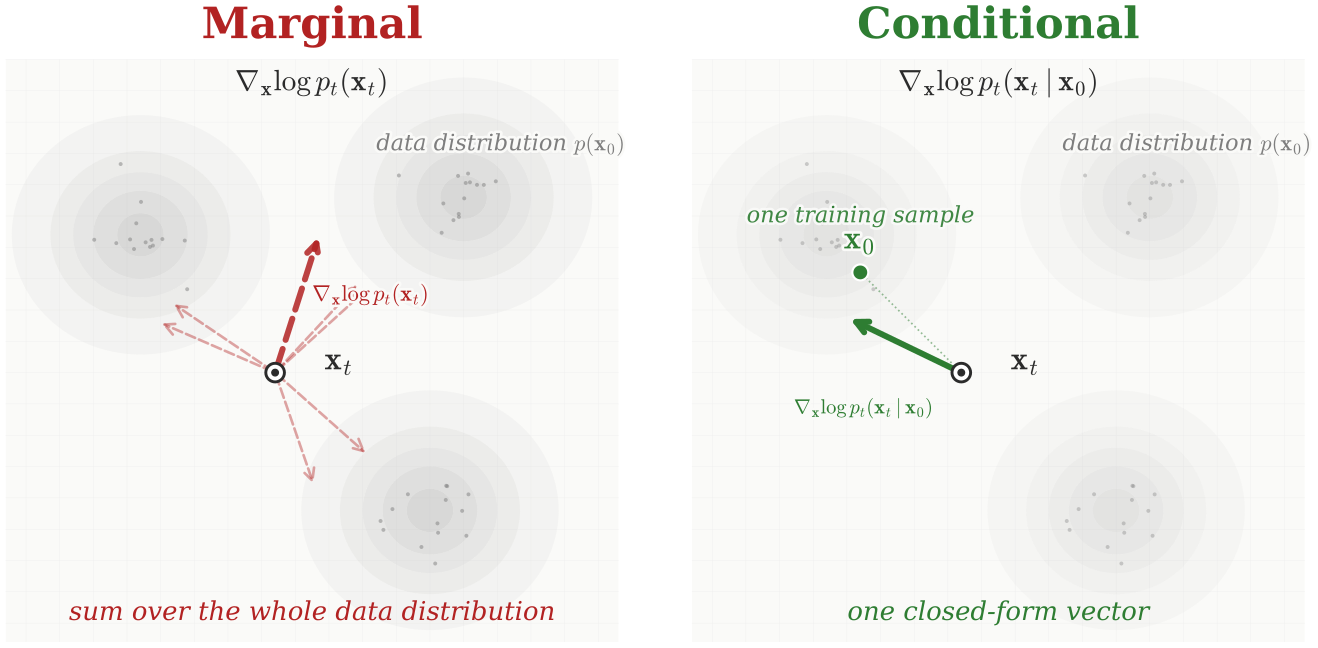
To avoid relying on the intractable oracle score \(\nabla_{{\mathbf{x}}} \log p_t({\mathbf{x}})\), the DSM loss in Equation in Chapter 3 is employed. Conditioned on a data point \({\mathbf{x}}_0\), this approach allows the use of the analytically tractable score \(\nabla_{{\mathbf{x}}_t} \log p_t({\mathbf{x}}_t|{\mathbf{x}}_0)\) via Equation in Appendix D, with concrete examples given in Section 1.4. Specifically, we exploit the following loss function:
\[\begin{equation} \label{eq:conti-dsm_loss-real} \begin{aligned} &\mathcal{L}_{\text{DSM}}(\bm{\phi}; \omega(\cdot)) := \\ &\frac{1}{2} \mathbb{E}_{t} \mathbb{E}_{{\mathbf{x}}_0} \mathbb{E}_{ p_t({\mathbf{x}}_t|{\mathbf{x}}_0)} \Big[\omega(t)\left\lVert\mathbf{s}_{\bm{\phi}}({\mathbf{x}}_t, t) - \nabla_{{\mathbf{x}}_t} \log p_t({\mathbf{x}}_t|{\mathbf{x}}_0)\right\rVert_2^2 \Big], \end{aligned} \end{equation}\]
where \({\mathbf{x}}_0 \sim p_{\mathrm{data}}\). Equation \(\eqref{eq:conti-dsm_loss-real}\) can be interpreted as the continuous-time counterpart of Equation in Chapter 3, with the summation in the discrete case replaced by integration.
Similar to the result in Theorem in Chapter 3 (Equivalence of L_SM and L_DSM), the minimizer of Equation \(\eqref{eq:conti-dsm_loss-real}\) is uniquely determined as follows:
Proposition: Minimizer of DSM
The minimizer \(\mathbf{s}^*\) satisfies \[\begin{align} \label{eq:optimal-score} \begin{aligned} \mathbf{s}^*({\mathbf{x}}_t, t) = \mathbb{E}_{{\mathbf{x}}_0 \sim p({\mathbf{x}}_0 | {\mathbf{x}}_t)} \big[ \nabla_{{\mathbf{x}}_t} \log p_t({\mathbf{x}}_t | {\mathbf{x}}_0) \big]= \nabla_{{\mathbf{x}}_t} \log p_t({\mathbf{x}}_t), \end{aligned} \end{align}\] for almost every \({\mathbf{x}}_t \sim p_t\) and \(t \in [0,T]\).
Proof for Proposition. DSM objective can be understood as a least-squares error problem. Specifically, at each time \(t\), the optimal score function is given by the conditional expectation of the gradient of the log conditional density, which, under Bayes’ rule, is equivalent to the gradient of the log marginal density. For a detailed proof, see Appendix Section (Minimizer of SM and DSM) in Appendix D. ■
Sampling and Inference
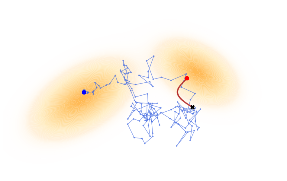
After learning \[\mathbf{s}_{\bm{\phi}^\times} := \mathbf{s}_{\bm{\phi}^\times}({\mathbf{x}}, t) \approx \nabla_{{\mathbf{x}}} \log p_t({\mathbf{x}}),\] we replace the intractable oracle score \(\nabla_{{\mathbf{x}}} \log p_t({\mathbf{x}})\) in the reverse-time SDE (Equation \(\eqref{eq:sde_backward}\)) and PF-ODE (Equation \(\eqref{eq:prob_ode_gt}\)) with the learned proxy \(\mathbf{s}_{\bm{\phi}^\times}({\mathbf{x}}, t)\). This substitution enables tractable inference via either the SDE or the ODE. For clarity, we distinguish the resulting processes as \({\mathbf{x}}^{\mathrm{SDE}}_{\bm{\phi}^\times}(t)\) and \({\mathbf{x}}^{\mathrm{ODE}}_{\bm{\phi}^\times}(t)\), respectively, but will omit this distinction in later sections.10
Empirical Reverse-Time SDE.
By substituting the trained score model \(\mathbf{s}_{\bm{\phi}^\times}\) for the true score in Equation \(\eqref{eq:sde_backward}\), we obtain the parameterized reverse-time SDE used for generation: \[\begin{equation} \label{eq:sde_backward_sub} \mathop{}\!\mathrm{d}{\mathbf{x}}^{\mathrm{SDE}}_{\bm{\phi}^\times}(t) = \left[\mathbf{f}\left({\mathbf{x}}^{\mathrm{SDE}}_{\bm{\phi}^\times}(t), t\right) - g^2(t) \mathbf{s}_{\bm{\phi}^\times}\left({\mathbf{x}}^{\mathrm{SDE}}_{\bm{\phi}^\times}(t), t\right) \right] \mathop{}\!\mathrm{d}t + g(t) \mathop{}\!\mathrm{d}\bar{{\mathbf{w}}}(t). \end{equation}\] To generate a sample, we first draw an initial value \({\mathbf{x}}_T\) from the prior distribution \(p_{\mathrm{prior}}\) and then numerically solve Equation \(\eqref{eq:sde_backward_sub}\) backward in time from \(t=T\) to \(t=0\). A standard numerical solver for this is the Euler–Maruyama method, which provides the discrete update rule: \[\begin{equation} \label{eq:euler-maruyama} {\mathbf{x}}_{t - \Delta t} \leftarrow {\mathbf{x}}_t - \left[ \mathbf{f}({\mathbf{x}}_t, t) - g^2(t) \mathbf{s}_{\bm{\phi}^\times}({\mathbf{x}}_t, t) \right] \Delta t + g(t) \sqrt{\Delta t} \cdot \boldsymbol{\epsilon}, \end{equation}\] where \(\boldsymbol{\epsilon} \sim \mathcal{N}(\bm{0}, \mathbf{I})\) and \(\Delta t > 0\) is the step size.
Iterating this update rule yields a final sample \({\mathbf{x}}^{\mathrm{SDE}}_{\bm{\phi}^\times}(0)\). If the score model is accurate, the distribution of these generated samples, denoted \(p_{\bm{\phi}^\times}^{\mathrm{SDE}}(\cdot; 0)\), provides a close approximation to the true data distribution11: \[p_{\bm{\phi}^\times}^{\mathrm{SDE}}(\cdot; 0) \approx p_{\mathrm{data}}(\cdot).\] Indeed, for the VP construction, the DDPM sampling scheme in Equation in Chapter 2 has the same continuous-time reverse-SDE limit as the Euler–Maruyama discretization above; see Section 1.4.
Empirical PF-ODE.
The PF-ODE defines a continuous flow connecting \(p_{\mathrm{prior}}\) and \(p_{\mathrm{data}}\), enabling sampling, encoding, and exact likelihood evaluation. The following section provides further details on each of these operations.
I. Sampling with PF-ODE.
Replacing the oracle score in Equation \(\eqref{eq:prob_ode_gt}\) with \(\mathbf{s}_{\bm{\phi}^\times}\) yields the empirical PF-ODE: \[\begin{equation} \label{eq:prob_ode_sub} \frac{\mathop{}\!\mathrm{d}}{\mathop{}\!\mathrm{d}t} {\mathbf{x}}^{\mathrm{ODE}}_{\bm{\phi}^\times}(t) = \mathbf{f}\left({\mathbf{x}}^{\mathrm{ODE}}_{\bm{\phi}^\times}(t), t\right) - \frac{1}{2} g^2(t) \mathbf{s}_{\bm{\phi}^\times}\left({\mathbf{x}}^{\mathrm{ODE}}_{\bm{\phi}^\times}(t), t\right). \end{equation}\] To generate samples, we begin by drawing an initial sample \({\mathbf{x}}_T\) from the prior distribution, \(p_{\mathrm{prior}}\). We then numerically solve the PF-ODE from Equation \(\eqref{eq:prob_ode_sub}\) backward in time from \(t=T\) to \(t=0\). This process is equivalent to approximating the integral: \[{\mathbf{x}}^{\mathrm{ODE}}_{\bm{\phi}^\times}(0) = {\mathbf{x}}_T + \int_T^0 \left[ \mathbf{f}\left({\mathbf{x}}^{\mathrm{ODE}}_{\bm{\phi}^\times}(\tau), \tau\right) - \frac{1}{2} g^2(\tau) \mathbf{s}_{\bm{\phi}^\times}\left({\mathbf{x}}^{\mathrm{ODE}}_{\bm{\phi}^\times}(\tau), \tau\right) \right] \mathrm{d}\tau.\] Solving this integral yields a final sample, \({\mathbf{x}}^{\mathrm{ODE}}_{\bm{\phi}^\times}(0)\). The distribution of samples generated via this deterministic process, denoted \(p_{\bm{\phi}^\times}^{\mathrm{ODE}}(\cdot; 0)\), provides an approximation to the data distribution, such that \(p_{\bm{\phi}^\times}^{\mathrm{ODE}}(\cdot; 0) \approx p_{\mathrm{data}}\).
Let \(\Delta t > 0\) denote a discretization step size. A standard numerical integration approach is the Euler method, which estimates \[\mathbf{f}({\mathbf{x}}_\tau, \tau) - \frac{1}{2} g^2(\tau) \mathbf{s}_{\bm{\phi}^\times}({\mathbf{x}}_\tau, \tau) \approx \mathbf{f}({\mathbf{x}}_t, t) - \frac{1}{2} g^2(t) \mathbf{s}_{\bm{\phi}^\times}({\mathbf{x}}_t, t), \quad \tau \in [t-\Delta t, t],\] leading to the following update rule: \[\begin{equation} \label{eq:euler-ode} {\mathbf{x}}_{t - \Delta t} \leftarrow {\mathbf{x}}_t - \left[ \mathbf{f}({\mathbf{x}}_t, t) - \frac{1}{2} g^2(t) \mathbf{s}_{\bm{\phi}^\times}({\mathbf{x}}_t, t) \right] \Delta t. \end{equation}\]
This connection allows us to reframe the process of generation with the following core insight:
Insight: Generation \(\Leftrightarrow\) ODE/SDE Solving
Sampling from diffusion models is fundamentally equivalent to solving a corresponding probability flow ODE or a reverse-time SDE.
This equivalence provides a clear explanation for the slow sampling speeds of diffusion models, as raised in Question ques:dm-sampling-slow. Generation is computationally intensive because numerical solvers for these differential equations are inherently iterative, often requiring many steps to accurately approximate a solution trajectory12. However, the PF-ODE formulation is also advantageous, as it allows us to leverage the extensive literature on accelerated numerical solvers. Exploring these techniques to speed up diffusion model sampling is the primary focus of Chapter 9.
II. Inversion with PF-ODE.
As discussed, unlike in the case of SDEs, we can solve the same Equation \(\eqref{eq:prob_ode_sub}\) both forward (from \(0\) to \(T\)) and reverse (from \(T\) to \(0\)) in time. When solving it forward, the ODE flow maps data to its (noisy) latent representations across all \(t \in [0,T]\), which plays a role of an encoder. This concept enables powerful applications for controllable generation, such as image translation and editing and beyond (Mokady et al. 2023; Su et al. 2022).
III. Log-Likelihood Evaluation via PF-ODE.
The PF-ODE also allows us to evaluate the likelihood of a data sample. Recall from Equation in Chapter 5 that, for an ODE, the change in log-density along a trajectory is determined by the divergence of its velocity field.
For the learned PF-ODE, define \[{\mathbf{v}}_{\bm{\phi}^\times}({\mathbf{x}},t) := {\mathbf{f}}({\mathbf{x}},t) -\frac{1}{2}g^2(t){\mathbf{s}}_{\bm{\phi}^\times}({\mathbf{x}},t).\] If \({\mathbf{x}}(t)\) evolves according to \[\frac{\mathop{}\!\mathrm{d}}{\mathop{}\!\mathrm{d}t}{\mathbf{x}}(t) = {\mathbf{v}}_{\bm{\phi}^\times}({\mathbf{x}}(t),t),\] then its log-density satisfies \[\frac{\mathop{}\!\mathrm{d}}{\mathop{}\!\mathrm{d}t} \log p^{\mathrm{ODE}}_{\bm{\phi}^\times}({\mathbf{x}}(t);t) = -\nabla_{{\mathbf{x}}}\cdot {\mathbf{v}}_{\bm{\phi}^\times}({\mathbf{x}}(t),t).\]
To evaluate the likelihood of an observed sample \({\mathbf{x}}_0\), we run the PF-ODE forward from \(t=0\) to \(t=T\), mapping \({\mathbf{x}}_0\) to a terminal point where the model density is the tractable prior. We can simultaneously track the log-density change by defining \[\delta(t) := \log p^{\mathrm{ODE}}_{\bm{\phi}^\times}({\mathbf{x}}(t);t) - \log p^{\mathrm{ODE}}_{\bm{\phi}^\times}({\mathbf{x}}_0;0).\] Thus, \(\delta(0)=0\), and the state and log-density change can be computed together through \[\begin{align} \label{eq:score-sde-likelihood} \frac{\mathop{}\!\mathrm{d}}{\mathop{}\!\mathrm{d}t} \begin{bmatrix} {\mathbf{x}}(t)\\ \delta(t) \end{bmatrix} = \begin{bmatrix} {\mathbf{v}}_{\bm{\phi}^\times}({\mathbf{x}}(t),t)\\ -\nabla_{{\mathbf{x}}}\cdot {\mathbf{v}}_{\bm{\phi}^\times}({\mathbf{x}}(t),t) \end{bmatrix}, \qquad \begin{bmatrix} {\mathbf{x}}(0)\\ \delta(0) \end{bmatrix} = \begin{bmatrix} {\mathbf{x}}_0\\ 0 \end{bmatrix}. \end{align}\]
After integrating to \(t=T\), the terminal density is \(p_{\mathrm{prior}}({\mathbf{x}}(T))\). Therefore, \[\log p^{\mathrm{ODE}}_{\bm{\phi}^\times}({\mathbf{x}}_0;0) = \log p_{\mathrm{prior}}({\mathbf{x}}(T)) - \delta(T).\] Equivalently, \[\log p^{\mathrm{ODE}}_{\bm{\phi}^\times}({\mathbf{x}}_0;0) = \log p_{\mathrm{prior}}({\mathbf{x}}(T)) + \int_0^T \nabla_{{\mathbf{x}}}\cdot {\mathbf{v}}_{\bm{\phi}^\times}({\mathbf{x}}(t),t) \,\mathop{}\!\mathrm{d}t.\] Thus, the same PF-ODE used for generation and inversion also provides a continuous change-of-variables formula for likelihood evaluation.
Instantiations of SDEs
Song et al. (2020) categorize the drift term \({\mathbf{f}}({\mathbf{x}}, t)\) and the diffusion term \(g(t)\) in the forward SDE into three types based on the behavior of the variance during evolution. Here, we focus on two commonly used types: the Variance Explosion (VE) SDE and Variance Preserving (VP) SDE. While it is possible to design custom noise schedulers, their design can substantially influence empirical performance. Table 1.1 summarizes these two SDE instantiations.
| VE SDE | VP SDE | ||
|---|---|---|---|
| \(\mathbf{f}({\mathbf{x}}, t)\) | \(\mathbf{0}\) | \(-\frac{1}{2}\beta(t){\mathbf{x}}\) | |
| \(g(t)\) | \(\sqrt{\frac{\mathop{}\!\mathrm{d}\sigma^2(t)}{\mathop{}\!\mathrm{d}t}}\) | \(\sqrt{\beta(t)}\) | |
| SDE | \(\mathop{}\!\mathrm{d}{\mathbf{x}}(t) = g(t) \mathop{}\!\mathrm{d}{\mathbf{w}}(t)\) | \(\mathop{}\!\mathrm{d}{\mathbf{x}}(t) = -\frac{1}{2}\beta(t) {\mathbf{x}}(t) \mathop{}\!\mathrm{d}t + \sqrt{\beta(t)} \mathop{}\!\mathrm{d}{\mathbf{w}}(t)\) | |
| \(p_t({\mathbf{x}}_t|{\mathbf{x}}_0)\) | \(\mathcal{N}\left({\mathbf{x}}_t ; {\mathbf{x}}_0, \left(\sigma^2(t) - \sigma^2(0)\right){\mathbf{I}}\right)\) | \(\mathcal{N}\left({\mathbf{x}}_t ; {\mathbf{x}}_0 e^{-\frac{1}{2}\int_{0}^{t} \beta(\tau)\mathop{}\!\mathrm{d}\tau}, {\mathbf{I}}- {\mathbf{I}}e^{-\int_{0}^{t} \beta(\tau)\mathop{}\!\mathrm{d}\tau}\right)\) | |
| \(p_{\mathrm{prior}}\) | \(\mathcal{N}(\bm{0}, \sigma^2(T){\mathbf{I}})\) | \(\mathcal{N}(\bm{0}, {\mathbf{I}})\) |
VE SDE
VE SDE has the following components:
Drift Term: A zero drift term \(\mathbf{f}=\bm{0}\).
Diffusion Term: \(g(t)=\sqrt{\frac{\mathop{}\!\mathrm{d}\sigma^2(t)}{\mathop{}\!\mathrm{d}t}}\) for some function \(\sigma(t)\).
The forward SDE then takes the following form: \[\begin{equation} \label{eq:vesde} \mathop{}\!\mathrm{d}{\mathbf{x}}(t) = \sqrt{\frac{\mathop{}\!\mathrm{d}\sigma^2(t)}{\mathop{}\!\mathrm{d}t}} \mathop{}\!\mathrm{d}{\mathbf{w}}(t). \end{equation}\] Similarly, the results from Section 1.4.3 imply the perturbation kernel for the VE SDE and suggest selecting an appropriate prior distribution:
Perturbation Kernel: \[\begin{align*} p_t({\mathbf{x}}_t | {\mathbf{x}}_0) &= \mathcal{N}\left({\mathbf{x}}_t ; {\mathbf{x}}_0, \left(\sigma^2(t) - \sigma^2(0)\right){\mathbf{I}}\right) \end{align*}\]
Prior Distribution: Assume that \(\sigma(t)\) is an increasing function for \(t \in [0,T]\) and that \(\sigma^2(T) \gg \sigma^2(0)\). The prior distribution is given by: \[p_{\mathrm{prior}} := \mathcal{N}(\bm{0}, \sigma^2(T){\mathbf{I}}).\]
A typical instance of a VE SDE is NCSN with the following design: \[\sigma(t):=\sigma_{\mathrm{min}}\left(\frac{\sigma_{\mathrm{max}}}{\sigma_{\mathrm{min}}} \right)^t,\quad \text{for } t\in(0,1],\] where \(\sigma_{\mathrm{min}}\) and \(\sigma_{\mathrm{max}}\) are pre-specified constants. Namely, the sequence of variances is designed as a geometric sequence. With this, NCSN is viewed as a discretized version of VE SDE, as discussed in Section 1.1.1.
VP SDE
Let \(\beta\colon [0,T] \rightarrow \mathbb{R}_{\geq 0 }\) be a non-negative function of \(t\). A VP SDE is defined with the following components:
Drift Term: A linear drift given by \(\mathbf{f}({\mathbf{x}}, t) = -\frac{1}{2}\beta(t){\mathbf{x}}\).
Diffusion Term: \(g(t) = \sqrt{\beta(t)}\).
Thus, the forward SDE is expressed as: \[\begin{align} \label{eq:forward-linear-sde} \mathop{}\!\mathrm{d}{\mathbf{x}}(t) = -\frac{1}{2}\beta(t) {\mathbf{x}}(t) \mathop{}\!\mathrm{d}t + \sqrt{\beta(t)} \mathop{}\!\mathrm{d}{\mathbf{w}}(t). \end{align}\]
Using the results from Section 1.4.3, we can derive the perturbation kernel for the VP SDE and select an appropriate prior distribution:
Perturbation Kernel: \[p_t({\mathbf{x}}_t|{\mathbf{x}}_0) = \mathcal{N}\left({\mathbf{x}}_t ; {\mathbf{x}}_0 e^{-\frac{1}{2}\int_{0}^{t} \beta(\tau)\mathop{}\!\mathrm{d}\tau}, {\mathbf{I}}- {\mathbf{I}}e^{-\int_{0}^{t} \beta(\tau)\mathop{}\!\mathrm{d}\tau}\right).\]
Prior Distribution: \(p_{\mathrm{prior}} := \mathcal{N}(\bm{0}, {\mathbf{I}})\).
We remark that since the perturbation kernel is a Gaussian with a known mean and covariance, we can apply Equation in Appendix D to compute its score function.
A classic example of a VP SDE is the DDPM, where the noise schedule \(\beta(t)\) is defined as: \[\beta(t) := \beta_{\mathrm{min}} + t(\beta_{\mathrm{max}} - \beta_{\mathrm{min}}), \quad \text{for all } t \in [0,1].\] Here, \(\beta_{\mathrm{min}}\) and \(\beta_{\mathrm{max}}\) are pre-defined constants. With this, DDPM can be interpreted as a discretization of the VP SDE, as discussed in Section 1.1.1.
(Optional) How Is the Perturbation Kernel \(p_t({\mathbf{x}}_t|{\mathbf{x}}_0)\) Derived?
If the drift term in the forward SDE Equation \(\eqref{eq:sde_forward}\) is linear in \({\mathbf{x}}\), taking the form \[\begin{align*} {\mathbf{f}}({\mathbf{x}}, t) = f(t) {\mathbf{x}}, \end{align*}\] for some scalar-valued, time-dependent function \(f(t) \in \mathbb{R}\), then Equation \(\eqref{eq:sde_forward}\) becomes a linear SDE: \[\mathop{}\!\mathrm{d}{\mathbf{x}}(t) = f(t){\mathbf{x}}(t) \mathop{}\!\mathrm{d}t + g(t) \mathop{}\!\mathrm{d}{\mathbf{w}}(t).\]
Even if the initial distribution \(p_{\mathrm{data}}\) is non-Gaussian, the linearity of the drift ensures that the conditional process remains Gaussian. In particular, for \(t>0\), the transition kernel admits the form: \[p_t( {\mathbf{x}}_t | {\mathbf{x}}_0 ) = \mathcal{N} \left( {\mathbf{x}}_t; {\mathbf{m}}(t), P(t) \mathbf{I}_D \right),\] where \({\mathbf{x}}_0 \sim p_{\mathrm{data}}\), and \({\mathbf{m}}(t) \in \mathbb{R}^D\), \(P(t)\in\mathbb{R}_{\ge 0}\) denote the conditional mean and (scalar) variance given \({\mathbf{x}}_0\), defined as: \[{\mathbf{m}}(t) = \mathbb{E} \left[{\mathbf{x}}_t | {\mathbf{x}}(0) = {\mathbf{x}}_0\right], \qquad P(t) \mathbf{I}_D = \operatorname{Cov} \left[{\mathbf{x}}_t | {\mathbf{x}}(0) = {\mathbf{x}}_0\right].\]
These first and second moments evolve according to the following ODEs (Särkkä and Solin 2019): \[\begin{align} \label{eq:mean-var-evolution} \begin{aligned} \frac{\mathop{}\!\mathrm{d}{\mathbf{m}}(t)}{\mathop{}\!\mathrm{d}t} &= f(t) {\mathbf{m}}(t), \\ \frac{\mathop{}\!\mathrm{d}P(t)}{\mathop{}\!\mathrm{d}t} &= 2f(t) P(t) + g^2(t), \end{aligned} \end{align}\] provided that the initial mean \({\mathbf{m}}(0)\) and variance \(P(0)\) are finite.
Since both ODEs are linear, they admit closed-form solutions via the integrating factor method. Given the initial condition \({\mathbf{x}}_0\), the mean and variance evolve as \[\begin{align} \label{eq:mean-var-solution} {\mathbf{m}}(t) = \mathcal{E}(0 \to t) {\mathbf{x}}_0, \qquad P(t) = \int_{0}^{t} \mathcal{E}^{2}(s \to t) g(s)^{2} \mathop{}\!\mathrm{d}s, \end{align}\] with \({\mathbf{m}}(0)={\mathbf{x}}_0\) and \(P(0)=0\). Here \(\mathcal{E}(s \to t)\) denotes the exponential integrating factor \[\mathcal{E}(s \to t) := \exp \left(\int_{s}^{t} f(u) \mathop{}\!\mathrm{d}u\right),\] which captures the accumulated effect of the drift from time \(s\) to \(t\). Consequently, the transition kernel \(p_t({\mathbf{x}}_t | {\mathbf{x}}_0)\) also admits a closed-form expression.
We defer the justification that the conditional covariance of \(p_t({\mathbf{x}}_t |{\mathbf{x}}_0)\) is isotropic, that is \(\operatorname{Cov}[{\mathbf{x}}_t | {\mathbf{x}}_0] = P(t) \mathbf I_D\) under a \(D\)-dimensional Wiener process with independent coordinates and diffusion \(g(t)\mathbf I_D\), as well as the derivation of Equation \(\eqref{eq:mean-var-evolution}\), to Section (Itô’s Formula Application: Closed-Form Solution of a Linear SDE) in Appendix C, which relies on Itô calculus.
Example: VE SDE’s Transition Kernel
In the special case of VE SDE: \({\mathbf{f}}\equiv 0\) and \(g(t) = \sqrt{\frac{\mathop{}\!\mathrm{d}\sigma^2(t)}{\mathop{}\!\mathrm{d}t}}\), the mean and covariance of the solution to the SDE evolve as follows.
\[\frac{\mathop{}\!\mathrm{d}{\mathbf{m}}(t)}{\mathop{}\!\mathrm{d}t} = 0, \quad \text{with} \quad {\mathbf{m}}(0) = {\mathbf{x}}_0 \Longrightarrow {\mathbf{m}}(t) = {\mathbf{x}}_0.\]
\[\frac{\mathop{}\!\mathrm{d}P(t)}{\mathop{}\!\mathrm{d}t} = \frac{\mathop{}\!\mathrm{d}\sigma^2(t)}{\mathop{}\!\mathrm{d}t}, \quad \text{with} \quad P(0) = 0 \Longrightarrow P(t) = \sigma^2(t) - \sigma^2(0).\] Therefore \[p_t({\mathbf{x}}_t | {\mathbf{x}}_0)=\mathcal{N} \left({\mathbf{x}}_t; {\mathbf{x}}_0, \big(\sigma^2(t)-\sigma^2(0)\big)\mathbf{I}_D\right).\]
Example: VP SDE’s Transition Kernel
In the VP SDE case with drift \({\mathbf{f}}({\mathbf{x}}, t) = -\tfrac{1}{2}\beta(t) {\mathbf{x}}\) and diffusion \(g(t) = \sqrt{\beta(t)}\):
\[\frac{\mathop{}\!\mathrm{d}{\mathbf{m}}}{\mathop{}\!\mathrm{d}t} = -\frac{1}{2}\beta(t) {\mathbf{m}}(t), \quad B(t) \mathrel{:=}\int_{0}^{t} \beta(s) \mathop{}\!\mathrm{d}s, \quad {\mathbf{m}}(t) = e^{-\frac{1}{2}B(t)} {\mathbf{x}}_0.\]
The variance satisfies \[\frac{\mathop{}\!\mathrm{d}P}{\mathop{}\!\mathrm{d}t} = -\beta(t) P(t) + \beta(t).\] Applying the integrating factor \(e^{B(t)}\) with \(B(t) = \int_0^t \beta(s) \mathop{}\!\mathrm{d}s\), we obtain \[\frac{\mathop{}\!\mathrm{d}}{\mathop{}\!\mathrm{d}t} \left[P(t)e^{B(t)}\right] = \beta(t) e^{B(t)}.\] Integrating both sides gives \[P(t) = 1 - e^{-B(t)}.\] Hence the covariance is isotropic with \[{\mathbf{P}}(t) = P(t) \mathbf I_D = \bigl(1 - e^{-B(t)}\bigr)\mathbf I_D.\]
\[p_t({\mathbf{x}}_t|{\mathbf{x}}_0) = \mathcal{N} \left( {\mathbf{x}}_t; \underbrace{e^{-\frac{1}{2} B(t)} {\mathbf{x}}_0}_{{\mathbf{m}}(t)}, \underbrace{\big(1 - e^{-B(t)}\big)\mathbf{I}_D}_{P(t)\mathbf{I}_D} \right), \quad B(t) = \int_0^t \beta(s) \mathop{}\!\mathrm{d}s.\]
A Direct View Through Accumulated Perturbation Kernels
DDPM and Score SDE are commonly introduced by specifying how noise is added locally in time: through discrete forward transitions \(p({\mathbf{x}}_t|{\mathbf{x}}_{t-\Delta t})\) in DDPM, or through a continuous-time SDE in Score SDE. For training, however, a particularly useful object is the accumulated perturbation kernel \[p_t({\mathbf{x}}_t|{\mathbf{x}}_0),\] which describes the distribution at time \(t\) directly conditioned on the original data sample. This is precisely the form that appears naturally in the DDPM and continuous-time denoising objectives Equation in Chapter 2 and Equation.
This suggests a complementary viewpoint: rather than beginning with the local noise injection and then deriving \(p_t({\mathbf{x}}_t|{\mathbf{x}}_0)\), we can specify the accumulated perturbation kernel directly. For the linear-Gaussian processes considered below, an admissible accumulated kernel determines the corresponding linear SDE, and vice versa. This viewpoint makes the amount of signal and noise at each time explicit, connects directly to practical training objectives, and will also provide a useful bridge to the probability-path viewpoint of Flow Matching in Chapter 5.
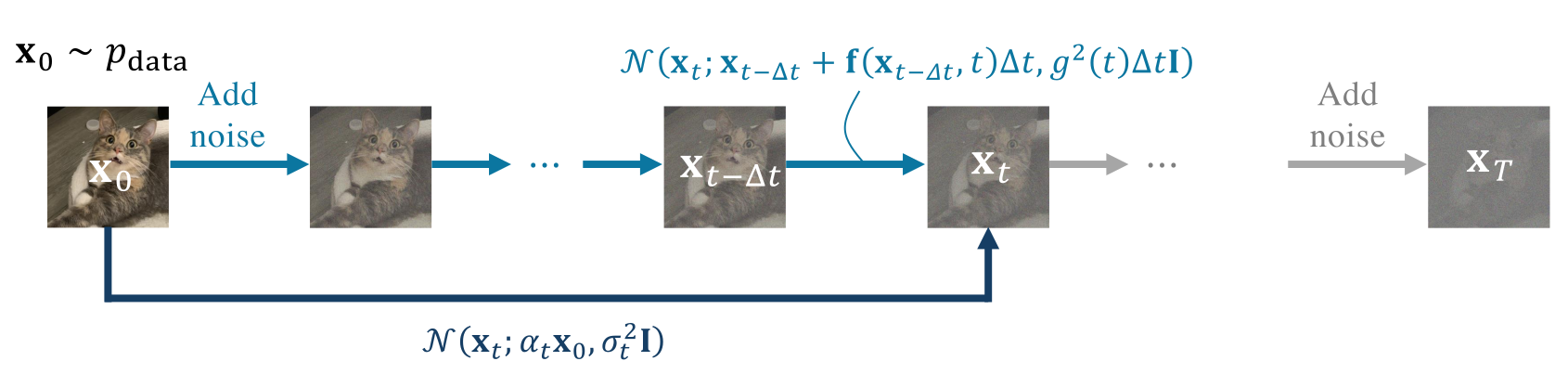
A General Affine Forward Process \(p_t({\mathbf{x}}_t|{\mathbf{x}}_0)\).
We begin by defining the accumulated forward perturbation kernel \[\begin{equation} \label{eq:forward_kernel} p_t({\mathbf{x}}_t|{\mathbf{x}}_0) := \mathcal{N}\bigl( {\mathbf{x}}_t; \alpha_t{\mathbf{x}}_0, \sigma_t^2\mathbf{I} \bigr), \end{equation}\] where \({\mathbf{x}}_0\sim p_{\mathrm{data}}\), and \(\alpha_t\) and \(\sigma_t\) are nonnegative scalar functions of \(t\in[0,T]\). In the standard forward diffusion setup, we take \[\alpha_0=1, \qquad \sigma_0=0,\] so that the process starts exactly from the data, and assume \(\alpha_t>0\) and \(\sigma_t>0\) for \(t\in(0,T]\) whenever the corresponding ratios are used.
Equivalently, a sample from Equation \(\eqref{eq:forward_kernel}\) can be written as \[{\mathbf{x}}_t = \alpha_t{\mathbf{x}}_0 + \sigma_t\bm{\epsilon}, \qquad \bm{\epsilon}\sim\mathcal{N}(\mathbf{0},\mathbf{I}).\]
This simple form includes several familiar probability paths:
VE (NCSN): \(\alpha_t\equiv1\), with the noise scale \(\sigma_t\) increasing over time;
VP (DDPM): \(\alpha_t^2+\sigma_t^2=1\);
Linear Gaussian interpolation: \(\alpha_t=1-t\) and \(\sigma_t=t\) on \(t\in[0,1]\), corresponding to the familiar linear path used in Flow Matching and Rectified Flow when written in the data-to-noise time convention.
Connection to Score SDE
For Score SDE, it is often more intuitive to specify the accumulated perturbation kernel \(p_t({\mathbf{x}}_t|{\mathbf{x}}_0)\) first and then recover the corresponding SDE coefficients, rather than starting from the drift and diffusion terms and solving ODEs for the moments (see Section 1.4.3).
For an admissible affine schedule, the corresponding forward SDE takes the linear-in-\({\mathbf{x}}\) form in Equation \(\eqref{eq:forward-linear-sde}\): \[\begin{align*} \mathop{}\!\mathrm{d}{\mathbf{x}}(t) = \underbrace{f(t){\mathbf{x}}(t)}_{{\mathbf{f}}({\mathbf{x}}(t),t)} \mathop{}\!\mathrm{d}t + g(t)\mathop{}\!\mathrm{d}{\mathbf{w}}(t), \end{align*}\] where \(f,g\colon[0,T]\rightarrow\mathbb{R}\) are real-valued functions of time.
The coefficients \(f(t)\) and \(g(t)\) can be recovered analytically from \(\alpha_t\) and \(\sigma_t\). Importantly, not every choice of \(\alpha_t\) and \(\sigma_t\) defines a valid diffusion: the implied diffusion variance \(g^2(t)\) must remain nonnegative. Equivalently, in this linear-Gaussian setting, the signal-to-noise ratio \(\alpha_t^2/\sigma_t^2\) cannot increase with time. The following lemma makes this relationship precise.
Lemma: Forward Perturbation Kernel \(\Leftrightarrow\) Linear SDE
Assume \(\alpha_0=1\), \(\sigma_0=0\), and that \(\alpha_t>0\) and \(\sigma_t>0\) are differentiable for \(t\in(0,T]\). Define \(\lambda_t:=\log\tfrac{\alpha_t}{\sigma_t}\).
Given the forward perturbation kernel \[{\mathbf{x}}_t=\alpha_t{\mathbf{x}}_0+\sigma_t{\bm{\epsilon}}, \qquad {\bm{\epsilon}}\sim\mathcal N(\mathbf 0,{\mathbf{I}}),\] there exists a corresponding linear SDE \[\mathop{}\!\mathrm{d}{\mathbf{x}}(t)=f(t){\mathbf{x}}(t)\mathop{}\!\mathrm{d}t+g(t)\mathop{}\!\mathrm{d}{\mathbf{w}}(t)\] with the same conditional kernel \(p_t({\mathbf{x}}_t|{\mathbf{x}}_0) =\mathcal N({\mathbf{x}}_t;\alpha_t{\mathbf{x}}_0,\sigma_t^2{\mathbf{I}})\) if and only if the coefficients \[\begin{align} \label{eq:kernel-sde-equiv} \begin{aligned} f(t) &=\frac{\mathop{}\!\mathrm{d}}{\mathop{}\!\mathrm{d}t}\log\alpha_t,\\ g^2(t) &=\frac{\mathop{}\!\mathrm{d}\sigma_t^2}{\mathop{}\!\mathrm{d}t} -2\frac{\mathop{}\!\mathrm{d}}{\mathop{}\!\mathrm{d}t}\log\alpha_t\,\sigma_t^2 =-2\sigma_t^2\frac{\mathop{}\!\mathrm{d}}{\mathop{}\!\mathrm{d}t}\lambda_t \end{aligned} \end{align}\] satisfy \(g^2(t)\geq 0\) for \(t\in(0,T]\). Equivalently, \(\lambda_t\) must be non-increasing.
Conversely, if a linear SDE has conditional kernels \(\mathcal N({\mathbf{x}}_t;\alpha_t{\mathbf{x}}_0,\sigma_t^2{\mathbf{I}})\) with \(\alpha_t>0\) and \(\sigma_t>0\), then its coefficients necessarily satisfy Equation \(\eqref{eq:kernel-sde-equiv}\).
Proof for Lemma. From Section 1.4.3, the result follows by matching the mean and covariance ODEs \({\mathbf{m}}'(t)=f(t){\mathbf{m}}(t)\) and \({\mathbf{P}}'(t)=2f(t){\mathbf{P}}(t)+g^2(t){\mathbf{I}}\) with \({\mathbf{m}}(t)=\alpha_t{\mathbf{x}}_0\) and \({\mathbf{P}}(t)=\sigma_t^2{\mathbf{I}}\). ■
Remark. To make the terminal conditional distribution independent of \({\mathbf{x}}_0\) and equal to a prescribed Gaussian prior, we need \(\alpha_T=0\) and \(\sigma_T^2\) equal to the prior variance. Since \[\alpha_t = \exp\Big(\int_0^t f(u)\mathop{}\!\mathrm{d}u\Big),\] achieving \(\alpha_T=0\) at a finite terminal time requires \[\int_0^T f(u)\mathop{}\!\mathrm{d}u=-\infty.\] Thus, the contraction induced by the drift must become singular near the terminal time; in particular, \(f\) cannot remain bounded on \([0,T]\).
The diffusion coefficient is related to the prescribed variance through \[g^2(t) = (\sigma_t^2)' - 2\frac{\alpha_t'}{\alpha_t}\sigma_t^2.\] For the usual regular schedules in which \(\sigma_t^2\) approaches a finite nonzero terminal variance, \((\sigma_t^2)'\) remains bounded, and \(\alpha_t'/\alpha_t\to-\infty\), this also gives \[g^2(t)\to\infty \qquad\text{as }t\to T.\] More generally, the precise behavior of \(g(t)\) depends on the chosen schedule.
If \(f\) and \(g\) remain bounded on a finite interval \([0,T]\), then \(\alpha_T>0\), so exact forgetting cannot occur at finite \(T\). In practice, one therefore chooses a terminal time for which the residual dependence on \({\mathbf{x}}_0\) is negligible and \(p_T\approx p_{\mathrm{prior}}\), or considers an infinite-time formulation in which \(\alpha_t\to 0\) asymptotically.
From the above lemma, specifying the incremental noise injection via a linear SDE with coefficients \(f(t)\) and \(g(t)\) is mathematically equivalent to defining the perturbation kernel with parameters \(\alpha_t\) and \(\sigma_t\). In the diffusion model literature, these two viewpoints are used interchangeably. Therefore, we conclude:
Observation
For a valid affine diffusion schedule, the two descriptions are equivalent: we may either specify the accumulated perturbation kernel \(p_t({\mathbf{x}}_t|{\mathbf{x}}_0)\) through \(\alpha_t\) and \(\sigma_t\), or specify the corresponding linear SDE through \(f(t)\) and \(g(t)\).
Connection to Variational-Based Diffusion Model
We revisit a core identity from DDPM, derived via Bayes’ rule: \[\begin{align} \label{eq:ddpm-reverse-condition-kernel} p({\mathbf{x}}_{t-\Delta t}|{\mathbf{x}}_t, {\mathbf{x}}) = p({\mathbf{x}}_t|{\mathbf{x}}_{t-\Delta t}) \cdot \frac{p_{t-\Delta t}({\mathbf{x}}_{t-\Delta t}|{\mathbf{x}})}{p_t({\mathbf{x}}_t|{\mathbf{x}})}, \end{align}\] for any \({\mathbf{x}}\) (usually \({\mathbf{x}}\sim p_{\mathrm{data}}\)). This reverse conditional \(p({\mathbf{x}}_{t-\Delta t} | {\mathbf{x}}_t, {\mathbf{x}})\) is central to modeling, enabling both tractable training targets and efficient sampling.
Although DDPM typically defines the incremental kernel \(p({\mathbf{x}}_t|{\mathbf{x}}_{t-\Delta t})\) first, the accumulated transition \(p_t({\mathbf{x}}_t|{\mathbf{x}}_0)\) often provides a more interpretable and practical formulation, especially for the prior and loss design.
Deriving Transition Kernels.
We now extend this to the continuous-time setting. Let \(0 \leq t < s \leq T\) be two (continuous) time points. Given the perturbation kernel \(p_t({\mathbf{x}}_t|{\mathbf{x}}_0)\), we can compute the reverse conditional \(p({\mathbf{x}}_t|{\mathbf{x}}_s, {\mathbf{x}})\) for any \({\mathbf{x}}\) by applying Equation \(\eqref{eq:ddpm-reverse-condition-kernel}\)13, using the forward kernel \(p({\mathbf{x}}_s|{\mathbf{x}}_t)\) as an intermediate. The following lemma summarizes this derivation, extending Lemma in Chapter 2 (Reverse Conditional Transition Kernel) without assuming \(\alpha_t^2 + \sigma_t^2 = 1\).
Lemma: Reverse Conditional Transition Kernels
Let \(0 \leq t < s \leq T\). The reverse conditional transition kernel is: \[\begin{equation*} p({\mathbf{x}}_t|{\mathbf{x}}_s, {\mathbf{x}}) = \mathcal{N}\left({\mathbf{x}}_t; \bm{\mu}({\mathbf{x}}_s, {\mathbf{x}}; s, t), \sigma^2(s, t) \mathbf{I}\right), \end{equation*}\] where \[\begin{align} \label{eq:p_backward_mean_var} \begin{aligned} \bm{\mu}({\mathbf{x}}_s, {\mathbf{x}}; s, t) := \frac{\alpha_{s|t} \sigma_t^2}{\sigma_s^2} {\mathbf{x}}_s + \frac{\alpha_t \sigma^2_{s|t}}{\sigma_s^2} {\mathbf{x}}, \quad \sigma^2(s, t) := \sigma^2_{s|t} \frac{\sigma_t^2}{\sigma_s^2}. \end{aligned} \end{align}\] Here, \(\alpha_{s|t}\) and \(\sigma_{s|t}\) are defined as: \[\begin{equation*} \alpha_{s|t} := \frac{\alpha_s}{\alpha_t}, \qquad \sigma^2_{s|t} := \sigma_s^2 - \alpha_{s|t}^2 \sigma_t^2. \end{equation*}\]
Proof for Lemma. We first compute the forward transition kernel: \[\begin{equation} \label{eq:zt_given_zs} p({\mathbf{x}}_s|{\mathbf{x}}_t) = \mathcal{N}\left({\mathbf{x}}_s; \alpha_{s|t} {\mathbf{x}}_t, \sigma^2_{s|t} \mathbf{I}\right). \end{equation}\] The reverse kernel then follows from Bayes’ rule, and since all involved distributions are Gaussian, the result can be derived by direct computation. For further details, see Appendix A of (Kingma et al. 2021). ■
Although \(p({\mathbf{x}}_{t + \Delta t}|{\mathbf{x}}_t)\) and \(p_t({\mathbf{x}}_t|{\mathbf{x}}_0)\) are theoretically equivalent, \(p_t({\mathbf{x}}_t|{\mathbf{x}}_0)\) often takes a more central role. The step-wise transition in Equation \(\eqref{eq:zt_given_zs}\) mainly serves to obtain a closed-form reverse kernel. Recent works (Kingma et al. 2021) thus favor directly specifying \(p_t({\mathbf{x}}_t|{\mathbf{x}}_0)\) for its clarity and interpretability.
Reverse Process Modeling, Training, and Sampling.
The training objective (ELBO in Equation in Chapter 2) and the modeling framework introduced in Section (Variational Perspective: DDPM) in Chapter 2 remain applicable under our generalized setting. For clarity, we adopt the \({\mathbf{x}}\)-prediction formulation, denoted by \({\mathbf{x}}_{\bm{\phi}}({\mathbf{x}}_s, s)\), following Kingma et al. (2021). However, the equivalent \({\bm{\epsilon}}\)-prediction perspective, represented by \(\bm{\epsilon}_{\bm{\phi}}({\mathbf{x}}_s, s)\), is also valid due to the relationship (as in Equation in Chapter 2) \[{\mathbf{x}}_s = \alpha_s {\mathbf{x}}_{\bm{\phi}}({\mathbf{x}}_s, s) + \sigma_s \bm{\epsilon}_{\bm{\phi}}({\mathbf{x}}_s, s),\quad \text{for any given } {\mathbf{x}}_s \sim q_s.\]
Modeling and Diffusion Loss \(\mathcal{L}_{\text{diffusion}}\).
Similar to DDPM, the conditional distribution \(p({\mathbf{x}}_t|{\mathbf{x}}_s, {\mathbf{x}})\) in Equation \(\eqref{eq:p_backward_mean_var}\) motivates replacing the clean signal \({\mathbf{x}}\) with a learnable predictor \({\mathbf{x}}_{\bm{\phi}}({\mathbf{x}}_s, s)\), yielding a parameterized reverse model of the form: \[\begin{align} \label{eq:general-ddpm-sampling} p_{\bm{\phi}}({\mathbf{x}}_t | {\mathbf{x}}_s) := \mathcal{N}\left({\mathbf{x}}_t; \bm{\mu}_{\bm{\phi}}({\mathbf{x}}_s, s, t), \sigma^2(s,t) \mathbf{I}\right), \end{align}\] with the mean parametrized as: \[\bm{\mu}_{\bm{\phi}}({\mathbf{x}}_s, s, t) = \frac{\alpha_{s|t} \sigma_t^2}{\sigma_s^2} {\mathbf{x}}_s + \frac{\alpha_t \sigma_{s|t}^2}{\sigma_s^2} {\mathbf{x}}_{\bm{\phi}}({\mathbf{x}}_s, s).\] Given the forward kernel in Equation \(\eqref{eq:forward_kernel}\), the KL divergence in \(\mathcal{L}_{\text{diffusion}}({\mathbf{x}}; \bm{\phi})\) reduces to a weighted regression loss: \[\begin{align} \begin{aligned} \label{eq:snr-kl} \mathcal{D}_{\text{KL}}\big(p({\mathbf{x}}_t|{\mathbf{x}}_s, {\mathbf{x}}_0) \| p_{\bm{\phi}}({\mathbf{x}}_t|{\mathbf{x}}_s)\big) &= \frac{1}{2\sigma^2(s,t)} \left\| \bm{\mu}({\mathbf{x}}_s, {\mathbf{x}}_0; s,t) - \bm{\mu}_{\bm{\phi}}({\mathbf{x}}_s, s, t) \right\|_2^2 \\ &= \frac{1}{2} \big(\text{SNR}(t) - \text{SNR}(s)\big) \left\| {\mathbf{x}}_0 - {\mathbf{x}}_{\bm{\phi}}({\mathbf{x}}_s, s) \right\|_2^2, \end{aligned} \end{align}\] where \({\mathbf{x}}_s = \alpha_s{\mathbf{x}}_0 + \sigma_s\bm{\epsilon}\), with \({\mathbf{x}}_0 \sim p_{\mathrm{data}}\), \(\bm{\epsilon} \sim \mathcal{N}(\bm{0}, {\mathbf{I}})\), and \(\text{SNR}(s) := \alpha_s^2 / \sigma_s^2\) denotes the signal-to-noise ratio at time \(s\).
Remark. In (Kingma et al. 2021), the authors study the continuous-time limit of Equation \(\eqref{eq:snr-kl}\) as \(t \to s\), yielding: \[\begin{align*} \mathcal{L}_{\text{VDM}}^\infty({\mathbf{x}}_0) = -\frac{1}{2} \mathbb{E}_{s, \bm{\epsilon} \sim \mathcal{N}(\bm{0}, \mathbf{I})} \text{SNR}'(s) \big\| {\mathbf{x}}_0 - {\mathbf{x}}_{\bm{\phi}}({\mathbf{x}}_s, s) \big\|_2^2. \end{align*}\] This setup also introduces a learnable noise schedule, and while it generalizes beyond continuous data, such extensions fall outside the scope of our current discussion.
Sampling.
Sampling proceeds similarly to DDPM using the parameterized kernel from Equation \(\eqref{eq:general-ddpm-sampling}\): \[\begin{align} \label{eq:general-ddpm-sampling-discrete} {\mathbf{x}}_t = \underbrace{\frac{\alpha_{s|t} \sigma_t^2}{\sigma_s^2} {\mathbf{x}}_s + \frac{\alpha_t \sigma_{s|t}^2}{\sigma_s^2} {\mathbf{x}}_{\bm{\phi}^\times}({\mathbf{x}}_s, s)}_{\bm{\mu}_{\bm{\phi}^\times}({\mathbf{x}}_s, t, s)} + \sigma_{s|t} \frac{\sigma_t}{\sigma_s} \bm{\epsilon}_s,\quad \bm{\epsilon}_s \sim \mathcal{N}(\bm{0}, {\mathbf{I}}). \end{align}\]
(Optional) Fokker–Planck Equation and
Reverse-Time SDEs
via Marginalization and Bayes’ Rule
In this section, we offer a probabilistic perspective on the structure of the Fokker–Planck equation and the reverse-time SDE. By leveraging fundamental tools such as the marginalization trick and Bayes’ rule, we illuminate the connection between the statistical formulation of stochastic processes and their corresponding differential equations.
We emphasize that the “derivation” presented here is not mathematically rigorous proofs, but rather heuristic arguments intended to convey the underlying connections.
Fokker-Planck Equation from the Marginalization of Transition Kernels
Given the forward transition probability as in Equation \(\eqref{eq:transition-forward-f-g}\) \[\begin{align*} p(\mathbf{x}_{t+\Delta t} | \mathbf{x}_t) = \mathcal{N}\left(\mathbf{x}_{t+\Delta t}; \mathbf{x}_t + \mathbf{f}(\mathbf{x}_t, t)\Delta t, g^2(t)\Delta t \mathbf{I}\right), \end{align*}\] and the marginal distributions \[\begin{align*} p_t(\mathbf{x}_t), \quad p_{t+\Delta t}(\mathbf{x}_{t+\Delta t}), \end{align*}\] we aim to derive the Fokker-Planck equation that governs the time evolution of the marginal distribution \(p_t\).
Change of Variables.
By the Markov property, the marginal distribution at time \(t + \Delta t\) can be expressed as an integral over the previous state \(\mathbf{x}_t\) (i.e., Chapman-Kolmogorov equation): \[\begin{align*} p_{t+\Delta t}({\mathbf{x}}) = \int \mathcal N \big({\mathbf{x}}; {\mathbf{y}}+{\mathbf{f}}({\mathbf{y}},t)\Delta t, g^2(t)\Delta t {\mathbf{I}}\big) p_t({\mathbf{y}}) \mathop{}\!\mathrm{d}{\mathbf{y}}. \end{align*}\] We introduce a new variable \[{\mathbf{u}}:= {\mathbf{y}}+{\mathbf{f}}({\mathbf{y}},t)\Delta t,\] so the Gaussian is centered at \({\mathbf{u}}\). For small \(\Delta t\), this map is invertible with \[{\mathbf{y}}= {\mathbf{u}}-{\mathbf{f}}({\mathbf{u}},t)\Delta t+\mathcal O(\Delta t^2), \quad \Bigg|\det\frac{\partial {\mathbf{y}}}{\partial {\mathbf{u}}}\Bigg| = 1-(\nabla_{\mathbf{u}}\cdot{\mathbf{f}})({\mathbf{u}},t) \Delta t+\mathcal O(\Delta t^2).\] Hence, change-of-variable formula leads us to: \[\begin{align*} p_{t+\Delta t}({\mathbf{x}}) &= \int \mathcal N\left({\mathbf{x}};{\mathbf{u}},g^2(t)\Delta t{\mathbf{I}}\right) \cdot \\\ quad\Big[p_t({\mathbf{u}})&-\Delta t {\mathbf{f}}({\mathbf{u}},t) \cdot \nabla_{\mathbf{u}}p_t({\mathbf{u}}) -\Delta t (\nabla_{\mathbf{u}}\cdot{\mathbf{f}})({\mathbf{u}},t) p_t({\mathbf{u}})\Big] \mathop{}\!\mathrm{d}{\mathbf{u}} +\mathcal O(\Delta t^2), \end{align*}\]
Taylor Expansion.
For any smooth function \(\phi:\mathbb{R}^D\to\mathbb{R}\) and scale \(\sigma>0\), if \({\mathbf{z}}\sim\mathcal N(\bm{0},{\mathbf{I}})\), the following approximation holds (known as the Taylor–Gaussian smoothing formula):
\[\int \mathcal N({\mathbf{x}};{\mathbf{u}},\sigma^2{\mathbf{I}}) \phi({\mathbf{u}}) \mathop{}\!\mathrm{d}{\mathbf{u}} =\mathbb{E}\left[\phi({\mathbf{x}}+\sigma{\mathbf{z}})\right] =\phi({\mathbf{x}})+\frac{\sigma^2}{2} \Delta_{\mathbf{x}}\phi({\mathbf{x}})+\mathcal O(\sigma^4).\] This is because Taylor expansion for: \[\phi({\mathbf{x}}+\sigma{\mathbf{z}})=\phi({\mathbf{x}})+\sigma\nabla_{\mathbf{x}}\phi({\mathbf{x}}) \cdot {\mathbf{z}}+\frac{\sigma^2}{2}{\mathbf{z}}^\top\nabla_{\mathbf{x}}^2\phi({\mathbf{x}}){\mathbf{z}}+\mathcal O(\sigma^3)\] and \(\mathbb{E}[{\mathbf{z}}]=\bm{0}\), \(\mathbb{E}[{\mathbf{z}}{\mathbf{z}}^\top]={\mathbf{I}}\).
Apply this with \(\phi=p_t\), \(\phi={\mathbf{f}}\cdot \nabla_{\mathbf{u}}p_t\), and \(\phi=(\nabla_{\mathbf{u}}\cdot{\mathbf{f}}) p_t\), and use \(\sigma^2=g^2(t)\Delta t\), we can obtain \[\begin{aligned} &p_{t+\Delta t}({\mathbf{x}}) - p_t({\mathbf{x}}) \\=& -\Delta t {\mathbf{f}}({\mathbf{x}},t) \cdot \nabla_{\mathbf{x}}p_t({\mathbf{x}}) -\Delta t (\nabla_{\mathbf{x}}\cdot{\mathbf{f}})({\mathbf{x}},t) p_t({\mathbf{x}}) +\frac{g^2(t)}{2}\Delta t \Delta_{\mathbf{x}}p_t({\mathbf{x}}) +\mathcal O(\Delta t^2) \\=& - \Delta t \nabla_{\mathbf{x}}\cdot \big({\mathbf{f}}({\mathbf{x}},t) p_t({\mathbf{x}})\big) + \frac{g^2(t)}{2} \Delta t \Delta_{\mathbf{x}}p_t({\mathbf{x}}) + \mathcal O(\Delta t^2). \end{aligned}\] Divide by \(\Delta t\) and let \(\Delta t\to0\) to obtain the Fokker–Planck equation.
In Section (Itô’s Formula’s Application: Derivation of Fokker-Planck Equation) in Appendix C, we present the Itô–based derivation to complement the discrete–time view above.
Why Does Reverse-Time SDE Take The Form?
The rigorous derivation of the reverse-time SDE is technical and requires delving into the properties of the Fokker-Planck equation. However, the form of the reverse-time SDE can be understood intuitively through Bayes’ theorem. Here, we present a heuristic derivation to provide insight into why Equation \(\eqref{eq:sde_backward}\) takes its form, with the appearance of score functions14.
Using Bayes’ Rule for Inversion.
Our goal is to determine the reverse-time transition kernel by first considering the discrete-time case: \[p({\mathbf{x}}_t | {\mathbf{x}}_{t+\Delta t}),\] and then taking \(\Delta t \rightarrow 0\) to obtain the continuous-time formulation. Using Bayes’ theorem, we express: \[\begin{align} \label{eq:reverse-sde-bayes-discrete} p({\mathbf{x}}_t | {\mathbf{x}}_{t+\Delta t}) &= p({\mathbf{x}}_{t+\Delta t} | {\mathbf{x}}_t) \frac{p_t({\mathbf{x}}_t)}{p_{t+\Delta t}({\mathbf{x}}_{t+\Delta t})} \nonumber \\ &= p({\mathbf{x}}_{t+\Delta t} | {\mathbf{x}}_t) \exp\left(\log p_t({\mathbf{x}}_t) - \log p_{t+\Delta t}({\mathbf{x}}_{t+\Delta t})\right). \end{align}\]
The forward transition kernel is assumed to be as in Equation \(\eqref{eq:transition-forward-f-g}\): \[\begin{equation*} p({\mathbf{x}}_{t+\Delta t} | {\mathbf{x}}_t) = \mathcal{N}\left({\mathbf{x}}_{t+\Delta t}; {\mathbf{x}}_t + {\mathbf{f}}({\mathbf{x}}_t, t)\Delta t, g^2(t)\Delta t \mathbf{I}\right) \end{equation*}\]
Taylor Expansion.
To handle the exponential term, we apply a first-order Taylor expansion. The key insight is to expand around the point \(({\mathbf{x}}_t, t)\) in both space and time: \[\begin{align*} \log p_{t+\Delta t}({\mathbf{x}}_{t+\Delta t}) &= \log p_t({\mathbf{x}}_t) + \nabla_{{\mathbf{x}}} \log p_t({\mathbf{x}}_t) \cdot ({\mathbf{x}}_{t+\Delta t} - {\mathbf{x}}_t) \nonumber \\ &\quad + \frac{\partial \log p_t({\mathbf{x}}_t)}{\partial t} \Delta t + \mathcal{O}(\|{\mathbf{h}}\|_2^2) \end{align*}\] where \({\mathbf{h}}:= ({\mathbf{x}}_{t+\Delta t} - {\mathbf{x}}_t, \Delta t)\). Therefore: \[\begin{align} \log p_t({\mathbf{x}}_t) - \log p_{t+\Delta t}({\mathbf{x}}_{t+\Delta t}) &= -\nabla_{{\mathbf{x}}} \log p_t({\mathbf{x}}_t) \cdot ({\mathbf{x}}_{t+\Delta t} - {\mathbf{x}}_t) \nonumber \\ &\quad - \frac{\partial \log p_t({\mathbf{x}}_t)}{\partial t} \Delta t + \mathcal{O}(\|{\mathbf{h}}\|_2^2) \label{eq:log-difference} \end{align}\]
For a diffusion process, \({\mathbf{x}}_{t+\Delta t}-{\mathbf{x}}_t=\mathcal O_p(\sqrt{\Delta t})\), so the second-order spatial Taylor terms are generally of order \(\mathcal O_p(\Delta t)\). Accordingly, the following calculation should be understood as a leading-order heuristic.
Substituting into the Reverse Transition.
Substituting equations Equation \(\eqref{eq:transition-forward-f-g}\) and Equation \(\eqref{eq:log-difference}\) into Equation \(\eqref{eq:reverse-sde-bayes-discrete}\): \[\begin{align*} &p({\mathbf{x}}_t | {\mathbf{x}}_{t+\Delta t}) \nonumber \\ = &\frac{1}{(2\pi g^2(t) \Delta t)^{D/2}} \exp\left(-\frac{\|{\mathbf{x}}_{t+\Delta t} - {\mathbf{x}}_t - {\mathbf{f}}({\mathbf{x}}_t, t) \Delta t\|_2^2}{2 g^2(t) \Delta t}\right) \nonumber \\ &\qquad \cdot \exp\left(-\nabla_{{\mathbf{x}}} \log p_t({\mathbf{x}}_t) \cdot ({\mathbf{x}}_{t+\Delta t} - {\mathbf{x}}_t) - \frac{\partial \log p_t({\mathbf{x}}_t)}{\partial t} \Delta t +\mathcal{O}(\Delta t)\right). \end{align*}\]
Algebraic Manipulation.
The key step is to complete the square in the exponent. We have: \[\begin{align*} &-\frac{\|{\mathbf{x}}_{t+\Delta t} - {\mathbf{x}}_t - {\mathbf{f}}({\mathbf{x}}_t, t) \Delta t\|_2^2}{2 g^2(t) \Delta t} - \nabla_{{\mathbf{x}}} \log p_t({\mathbf{x}}_t) \cdot ({\mathbf{x}}_{t+\Delta t} - {\mathbf{x}}_t) \nonumber \\ = &-\frac{\left[\|{\mathbf{x}}_{t+\Delta t} - {\mathbf{x}}_t - {\mathbf{f}}({\mathbf{x}}_t, t) \Delta t\|_2^2 + 2 g^2(t) \Delta t \nabla_{{\mathbf{x}}} \log p_t({\mathbf{x}}_t) \cdot ({\mathbf{x}}_{t+\Delta t} - {\mathbf{x}}_t)\right]}{2 g^2(t) \Delta t} \end{align*}\] Let \(\boldsymbol{\delta} := {\mathbf{x}}_{t+\Delta t} - {\mathbf{x}}_t\) and \(\boldsymbol{\mu} := {\mathbf{f}}({\mathbf{x}}_t, t) \Delta t\). Then: \[\begin{align*} &\|\boldsymbol{\delta} - \boldsymbol{\mu}\|_2^2 + 2 g^2(t) \Delta t \nabla_{{\mathbf{x}}} \log p_t({\mathbf{x}}_t) \cdot \boldsymbol{\delta} \nonumber \\ = &\|\boldsymbol{\delta}\|_2^2 - 2\boldsymbol{\delta} \cdot \boldsymbol{\mu} + \|\boldsymbol{\mu}\|_2^2 + 2 g^2(t) \Delta t \nabla_{{\mathbf{x}}} \log p_t({\mathbf{x}}_t) \cdot \boldsymbol{\delta} \nonumber \\ = &\|\boldsymbol{\delta}\|_2^2 - 2\boldsymbol{\delta} \cdot [\boldsymbol{\mu} - g^2(t) \Delta t \nabla_{{\mathbf{x}}} \log p_t({\mathbf{x}}_t)] + \|\boldsymbol{\mu}\|_2^2 \nonumber \\ = &\|\boldsymbol{\delta} - [\boldsymbol{\mu} - g^2(t) \Delta t \nabla_{{\mathbf{x}}} \log p_t({\mathbf{x}}_t)]\|_2^2 - \|g^2(t) \Delta t \nabla_{{\mathbf{x}}} \log p_t({\mathbf{x}}_t)\|_2^2 \end{align*}\] Substituting back: \[\begin{align*} &\|\boldsymbol{\delta} - [{\mathbf{f}}({\mathbf{x}}_t, t) \Delta t - g^2(t) \Delta t \nabla_{{\mathbf{x}}} \log p_t({\mathbf{x}}_t)]\|_2^2 \nonumber \\ = &\|{\mathbf{x}}_{t+\Delta t} - {\mathbf{x}}_t - [{\mathbf{f}}({\mathbf{x}}_t, t) - g^2(t) \nabla_{{\mathbf{x}}} \log p_t({\mathbf{x}}_t)] \Delta t\|_2^2. \end{align*}\] Therefore, \[\begin{align*} p({\mathbf{x}}_t | {\mathbf{x}}_{t+\Delta t}) =~&\frac{1}{(2\pi g^2(t) \Delta t)^{D/2}} \nonumber \\ \quad &\cdot \exp\left(-\frac{\|{\mathbf{x}}_{t+\Delta t} - {\mathbf{x}}_t - [{\mathbf{f}}({\mathbf{x}}_t, t) - g^2(t) \nabla_{{\mathbf{x}}} \log p_t({\mathbf{x}}_t)] \Delta t\|_2^2}{2 g^2(t) \Delta t}\right) \nonumber \\ \quad &\cdot \exp(\mathcal{O}(\Delta t)) \nonumber \\ =~&\mathcal{N}\left({\mathbf{x}}_t; {\mathbf{x}}_{t+\Delta t} - [{\mathbf{f}}({\mathbf{x}}_t, t) - g^2(t) \nabla_{{\mathbf{x}}} \log p_t({\mathbf{x}}_t)] \Delta t, g^2(t) \Delta t \mathbf{I}\right) \nonumber \\ \quad &\cdot (1 + \mathcal{O}(\Delta t)). \end{align*}\] The additional term \(\|g^2(t) \Delta t \nabla_{{\mathbf{x}}} \log p_t({\mathbf{x}}_t)\|_2^2\) from completing the square is \(\mathcal{O}((\Delta t)^2)\) and can be absorbed into the error term. Similarly, the time derivative term \(\frac{\partial \log p_t({\mathbf{x}}_t)}{\partial t} \Delta t\) is \(\mathcal{O}(\Delta t)\) and will vanish in the continuous limit.
Taking \(\Delta t \rightarrow 0\) Limit.
As \(\Delta t \approx 0\), under smoothness assumptions, the following approximations hold: \[\begin{align*} {\mathbf{f}}({\mathbf{x}}_t, t) &\approx {\mathbf{f}}({\mathbf{x}}_{t+\Delta t}, t+\Delta t), \\ g(t) &\approx g(t+\Delta t), \\ \nabla_{{\mathbf{x}}} \log p_t({\mathbf{x}}_t) &\approx \nabla_{{\mathbf{x}}} \log p_{t+\Delta t}({\mathbf{x}}_{t+\Delta t}) = {\mathbf{s}}({\mathbf{x}}_{t+\Delta t}, t+\Delta t). \end{align*}\] Using these approximations and some rearrangements, we obtain: \[\begin{align*} &p({\mathbf{x}}_t | {\mathbf{x}}_{t+\Delta t}) \\ \approx &\frac{1}{(2\pi g^2(t) \Delta t)^{D/2}} \exp \Bigg( \\ &-\frac{\Big\|{\mathbf{x}}_{t} - \Big({\mathbf{x}}_{t+\Delta t} - \big[{\mathbf{f}}({\mathbf{x}}_{t+\Delta t}, t+\Delta t) - g^2({t+\Delta t}) {\mathbf{s}}({\mathbf{x}}_{t+\Delta t}, t+\Delta t)\big] \Delta t\Big) \Big\|_2^2 }{2 g^2(t+\Delta t) \Delta t} \\ &\Bigg). \end{align*}\] This implies that \(p({\mathbf{x}}_t | {\mathbf{x}}_{t+\Delta t})\) is roughly a normal distribution with: \[\begin{align*} \mathbf{Mean:} & \quad{\mathbf{x}}_{t+\Delta t} - \big[{\mathbf{f}}({\mathbf{x}}_{t+\Delta t}, t+\Delta t) - g^2(t+\Delta t) {\mathbf{s}}({\mathbf{x}}_{t+\Delta t}, t+\Delta t)\big] \Delta t, \\ \mathbf{Covariance:} & \quad g^2(t+\Delta t) \Delta t \mathbf{I}. \end{align*}\] Taking the limit as \(\Delta t \rightarrow 0\), we “derive” the reverse-time continuous SDE given in Equation \(\eqref{eq:sde_backward}\).
Closing Remarks
This chapter marked a pivotal moment in our journey, unifying the discrete-time diffusion processes from the variational and score-based perspectives into a single, elegant continuous-time framework. We demonstrated that both DDPM and NCSN can be understood as discretizations of Stochastic Differential Equations (SDEs) with different drift/volatility coefficients.
The cornerstone of this framework is the existence of a corresponding reverse-time SDE, which formally defines a generative process that reverses the noise corruption. Crucially, the drift of this reverse process depends on a single unknown quantity: the score function, \(\nabla_{\mathbf{x}}\log{p_{t}(\mathbf{x})}\), of the marginal data distributions at every point in time. This insight solidifies the score function’s central role in generative modeling.
Furthermore, we introduced a purely deterministic counterpart, the Probability Flow Ordinary Differential Equation (PF-ODE), whose solution trajectories evolve along the same marginal densities \(\{p_{t}\}\) as the SDEs. This remarkable consistency is guaranteed by the underlying Fokker-Planck equation. The profound implication is that the complex task of generation is fundamentally equivalent to solving a differential equation. Training reduces to learning the score function that defines the equation’s vector field, while sampling becomes a problem of numerical integration.
The introduction of the PF-ODE, a purely deterministic flow, provides a powerful bridge to the third and final perspective on diffusion models. This concept of learning a deterministic transformation governed by a velocity field is the central principle of recent major family of generative models. In the next chapter, we will:
Explore this flow-based perspective, starting from its origins in Normalizing Flows and Neural ODEs.
Show how this viewpoint leads to the modern framework of Flow Matching, which directly learns a velocity field to transport samples between distributions.
Ultimately, we will see how the deterministic PF-ODE, which we derived from stochastic principles, can be constructed and generalized from this entirely different, flow-based origin, completing our unified picture of diffusion modeling.
In Section (Variational Perspective: DDPM) in Chapter 2, the DDPM forward step is written as \({\mathbf{x}}_i = \sqrt{1-\beta_i^2}\,{\mathbf{x}}_{i-1} + \beta_i\,\bm{\epsilon}_i\), where \(\beta_i\) denotes the standard deviation of the injected noise and \(\alpha_i := \sqrt{1-\beta_i^2}\). Here and throughout this chapter, we follow the convention of Song et al. (2020), where \(\beta_i\) instead denotes the variance of the injected noise, so that \({\mathbf{x}}_i = \sqrt{1-\beta_i}\,{\mathbf{x}}_{i-1} + \sqrt{\beta_i}\,\bm{\epsilon}_i\). The two conventions are related by \(\beta_i^{\mathrm{(here)}} = \bigl(\beta_i^{\mathrm{(Ch.\ 2)}}\bigr)^2\) and yield identical dynamics.↩︎
For convenience, we use \({\mathbf{x}}(t)\) and \({\mathbf{x}}_t\) interchangeably (and similarly for other time-dependent variables) to denote samples at time \(t\).↩︎
The forward kernel in Equation \(\eqref{eq:transition-forward-f-g}\) converges, as \(\Delta t\to0\), to the solution of the corresponding Itô SDE. A fully rigorous proof relies on advanced results which we defer to the literature.↩︎
Technically, this corresponds to solving the ODE with a time-flipping substitution \(t \leftrightarrow T - t\).↩︎
Naively flipping time does not yield the correct reverse process.↩︎
We use the “bar” notation to distinguish the reverse process \(\{ \bar{{\mathbf{x}}}(t) \}_{t \in [0, T]}\) from the forward process \(\{ {\mathbf{x}}(t) \}_{t \in [0, T]}\), defined by the forward-time SDE.↩︎
We use a tilde to distinguish processes associated with the forward and reverse-time SDEs. Going forward, we omit this notational distinction for simplicity.↩︎
The physical idea underlying this map is much older. Eighteenth-century fluid mechanics already studied motion through velocity fields and by following the evolution of material particles, notably in the foundational works of Euler and Lagrange (Euler 1757; Lagrange 1783).↩︎
Spoiler: the PF-ODE flow map \({\bm{\Psi}}_{s\to t}\) is exactly the Normalizing Flow (NF) bijection carrying \(p_s\) to \(p_t\) (to be detailed in Section (Flow-Based Models: Normalizing Flows and Neural ODEs) in Chapter 5). The difference is that, once the forward SDE and its marginal densities are fixed, the PF-ODE formula uniquely specifies its associated velocity field, \({\mathbf{v}}({\mathbf{x}},t) = {\mathbf{f}}({\mathbf{x}},t) -\frac{1}{2}g^2(t)\nabla_{{\mathbf{x}}}\log p_t({\mathbf{x}})\), whereas a normalizing flow, or continuous-time normalizing flow, parameterizes and learns a velocity field directly. Both rely on the same continuous change-of-variables principle.↩︎
This is to simplify notation after this subsection.↩︎
Theoretically, estimation accuracy depends on the discrepancy between \(p_T\) and \(p_{\mathrm{prior}}\) (typically negligible), model training error, and numerical discretization error (De Bortoli 2022; Wang et al. 2024). We do not pursue formal bounds here.↩︎
For example, DDPM and Score SDE typically use \(1,000\) function evaluations for generation.↩︎
This identity extends naturally to continuous time by treating \(s\) as a general earlier time.↩︎