Chapter 10: Distillation-Based Methods for Fast Sampling

This chapter introduces training-based approaches that accelerate diffusion model sampling by teaching new generators to produce samples in only one or a few steps. The central idea, called distillation, is to let a fast student model learn from a slow, pre-trained diffusion model (teacher) sampler. While the teacher may require hundreds of steps, the student can achieve comparable quality in only a few steps¹. Unlike solver-based acceleration, which improves the numerical integration scheme, distillation directly trains a generator to take efficient shortcuts. We highlight two main paradigms: distribution level distillation, which skips simulating the full trajectory and instead aligns the student’s output distribution with the teacher’s, and flow map level distillation, which trains the student to reproduce the teacher’s sampling path in a faster and more compact way.

Prologue

A central bottleneck of diffusion models is their slow sampling speed.

As shown through Tweedie’s formula (Section (Four Prediction Types Are Equivalent) in Chapter 6), a diffusion model can be interpreted as an “\({\mathbf{x}}\)-prediction” model, \({\mathbf{x}}_{\bm{\phi}^\times}({\mathbf{x}}_t, t)\), trained to recover the expected clean data from a noisy input \({\mathbf{x}}_t\) at noise level \(t\): \[{\mathbf{x}}_{\bm{\phi}^\times}({\mathbf{x}}_t, t) \approx \mathbb{E}[{\mathbf{x}}_0 |{\mathbf{x}}_t],\] where the expectation is taken with respect to \(p({\mathbf{x}}_0 |{\mathbf{x}}_t)\), representing all plausible clean data corresponding to \({\mathbf{x}}_t\). A natural idea is to use \({\mathbf{x}}_{\bm{\phi}^\times}({\mathbf{x}}_t, t)\) for one step generation. Yet because this denoiser averages over many plausible outcomes, the prediction can become overly smooth, and generation with only a few denoising steps leads to blurry, low quality samples.

On the other hand, as discussed in Section (Sampling and Inference) in Chapter 4, diffusion sampling follows an ODE or SDE trajectory through a long sequence of iterative steps. This produces high fidelity samples, but repeated neural-network evaluations make sampling expensive. For a deterministic ODE solver of order \(n\), under standard regularity assumptions, the local truncation error is \(\mathcal{O}(h^{n+1})\) and the global discretization error over a fixed time interval is \(\mathcal{O}(h^n)\), where \(h=\max_i |t_i-t_{i-1}|\) is the step size. Thus, using a coarser discretization generally increases numerical error for a fixed learned vector field, although sample fidelity need not decrease monotonically with the number of solver steps. This creates a practical trade off between sampling accuracy and computational cost.

To overcome this bottleneck, a major line of research is distillation, which assumes access to a well-trained diffusion model (the teacher) and trains a generator (the student) to reproduce its behavior through a single feed forward or few step computation. This compresses the teacher’s many sampling steps into a fast process, effectively bypassing slow iterative solvers while maintaining high sample fidelity.

Below, we introduce two perspectives on distillation: distribution level distillation and flow map level distillation².

Distribution Level Distillation

The goal of distribution-based distillation is to train a one-step generator \({\mathbf{G}}_{\bm{\theta}}({\mathbf{z}})\) that maps noise \({\mathbf{z}}\sim p_{\mathrm{prior}}\) to a sample \(\hat{\mathbf{x}}= {\mathbf{G}}_{\bm{\theta}}({\mathbf{z}})\), inducing a distribution \(p_{\bm{\theta}}(\hat{\mathbf{x}})\) that approximates the target data distribution \(p_{\mathrm{data}}({\mathbf{x}})\). This is typically achieved by minimizing a statistical divergence \[\min_{\bm{\theta}} \mathcal{D}\!\left(p_{\bm{\theta}}(\hat{\mathbf{x}}), p_{\mathrm{data}}(\hat{\mathbf{x}})\right),\] where \(\mathcal{D}\) denotes a suitable divergence measurement such as KL.

In practice, distribution based methods align the generator’s distribution with the empirical distribution \(p_{\bm{\phi}^\times}({\mathbf{x}})\) produced by a pre-trained diffusion model: \[\min_{\bm{\theta}} \mathcal{D}\!\left(p_{\bm{\theta}}(\hat{\mathbf{x}}), p_{\bm{\phi}^\times}(\hat{\mathbf{x}})\right),\] where \(p_{\bm{\phi}^\times}\) serves as a surrogate for \(p_{\mathrm{data}}\). Rather than evaluating this divergence explicitly, these methods construct tractable estimators of its gradient using the pre-trained teacher together with quantities estimated from the student’s current distribution. For KL-based distribution matching, this gradient takes the form of a difference between the student and target score functions.

This formulation distills multi-step generative processes of diffusion models into a single step model through distributional alignment. We detail this approach in Section 1.2.

Flow Map Level Distillation

We consider the PF-ODE, which can be expressed for any prediction model (see Equation in Chapter 6): \[\begin{align} \label{eq:pf-ode-ct} \frac{\mathop{}\!\mathrm{d}{\mathbf{x}}(\tau)}{\mathop{}\!\mathrm{d}\tau} = f(\tau) {\mathbf{x}}(\tau) - \tfrac{1}{2}g^2(\tau) \nabla_{\mathbf{x}}\log p_\tau({\mathbf{x}}(\tau)) =: {\mathbf{v}}^*({\mathbf{x}}(\tau), \tau). \end{align}\]

Its solution map (flow map), starting from \({\mathbf{x}}_s\) at time \(s\) and evolving reversely to time \(t \leq s\), is denoted by \({\bm{\Psi}}_{s\to t}({\mathbf{x}}_s)\); that is, \[\begin{align} \label{eq:int_target_gt} \begin{aligned} {\bm{\Psi}}_{s\to t}({\mathbf{x}}_s) &\mathrel{:=}{\mathbf{x}}_s + \int_s^t {\mathbf{v}}^*({\mathbf{x}}(\tau), \tau) \mathop{}\!\mathrm{d}\tau, \end{aligned} \end{align}\] where the integral solves the PF-ODE. Intuitively, \({\bm{\Psi}}_{s\to t}\) transports, \({\mathbf{x}}_s\), noise at time \(s\) to less noisy states at time \(t\) (ultimately data at \(t=0\)).

Sampling from a diffusion model corresponds to evaluating \({\bm{\Psi}}_{T\to 0}({\mathbf{x}}_T)\) for \({\mathbf{x}}_T \sim p_{\mathrm{prior}}\). Typically, this integral is approximated by iterative numerical solvers leveraging the velocity field \({\mathbf{v}}\) (see Chapter 9), but requires many steps (e.g., at least \(10\)-\(20\) NEFs even in DPM-Solver), making sampling slower than classic one-step generative models such as GAN. This motivates a natural question:

In particular, learning a map \({\bm{\Psi}}_{T\to 0}({\mathbf{x}}_T)\) with \({\mathbf{x}}_T \sim p_{\mathrm{prior}}\) enables one-step generation.

Trajectory Distillation.

Trajectory distillation seeks to train a neural generator that approximates the solution map at the instance level. Since the PF-ODE integral rarely admits a closed form, it must be approximated numerically during training. To formalize, we introduce the general solver notation \[\begin{align} \label{eq:solver} \mathtt{Solver}_{s\to t}({\mathbf{x}}_s;\,\bm{\phi}^\times) \quad \text{or simply} \quad \mathtt{Solver}_{s\to t}({\mathbf{x}}_s), \end{align}\] denoting numerical integration of the empirical PF-ODE from \(s\) to \(t\) starting at \({\mathbf{x}}_s\), with teacher parameters \(\bm{\phi}^\times\) (omitted when clear from context).

An Early Approach: Direct Knowledge Distillation.

To enable few step or even one step generation, a direct approach is to train a generator \({\mathbf{G}}_{\bm{\theta}}({\mathbf{x}}_T, T,0)\) to imitate the output of a numerical solver evaluated along the full trajectory: \[{\mathbf{G}}_{\bm{\theta}}({\mathbf{x}}_T, T,0)\approx \mathtt{Solver}_{T\to 0}({\mathbf{x}}_T), \qquad {\mathbf{x}}_T \sim p_{\mathrm{prior}}.\] This idea underlies one of the earliest trajectory distillation methods, Knowledge Distillation (Luhman and Luhman 2021), which uses the regression loss \[\mathcal{L}_{\mathrm{KD}}({\bm{\theta}}) := \mathbb{E}_{{\mathbf{x}}_T \sim p_{\mathrm{prior}}} \left\| {\mathbf{G}}_{\bm{\theta}}({\mathbf{x}}_T, T,0) - \mathtt{Solver}_{T\to 0}({\mathbf{x}}_T) \right\|_2^2.\] While this approach provides direct supervision from the pre-trained teacher, it cannot leverage the strong supervision available in the original training data. In addition, it is computationally expensive if ODE integration is invoked within the training loop, since each parameter update requires solving the ODE to form targets. Finally, because the generator learns only a global mapping from \(T\) to \(0\), it may lose controllability for steering the generation process from intermediate states. Consequently, most controllable generation techniques introduced in Chapter 8 cannot be directly applied.

Preface to Progressive Distillation.

Progressive Distillation (PD) (Salimans and Ho 2021) trains a time–conditional \(\mathtt{Student}\) using local supervision from \(\mathtt{Teacher}\) fragments. Let \(t_0=T>t_1>\cdots>t_N=0\) be a fixed time grid. The \(\mathtt{Teacher}\) provides time–stepping maps \(\mathtt{Teacher}_{t_k\to t_{k+1}}\) for \(k=0,\ldots,N-1\).

Rather than supervising only the one-jump \(T\to 0\), PD trains the \(\mathtt{Student}\) two–step skip map to match two consecutive \(\mathtt{Teacher}\) steps: \[\mathtt{Student}_{t_k\to t_{k+2}} \;\approx\; \mathtt{Teacher}_{t_{k+1}\to t_{k+2}} \circ \mathtt{Teacher}_{t_{k}\to t_{k+1}},\] for \(k = 0, 2, 4, \dots\). The matching is performed using a simple regression loss (e.g., mean squared error).

After training on locally paired fragments, the \(\mathtt{Student}\) no longer follows every time interval of the original grid. Instead, it advances on every other time point, \[t_0 \to t_2 \to t_4 \to \cdots \to t_N,\] which means that each \(\mathtt{Student}\) step effectively covers two consecutive \(\mathtt{Teacher}\) steps. Consequently, the \(\mathtt{Student}\) completes the same overall time span \([0,T]\) using only \(N/2\) transitions.

After this stage, the trained \(\mathtt{Student}\) replaces the \(\mathtt{Teacher}\) to serve as the new reference model. The entire procedure is then repeated on the coarser grid, where the time step doubles \((N \to N/2 \to N/4 \to \cdots)\), progressively distilling the trajectory into fewer and fewer steps until the desired number of inference steps is reached. This iterative halving preserves the global time horizon while continually compressing the temporal resolution of the generative process.

A Unified Perspective of Flow Map Learning.

Various methods, including KD and PD, can be expressed within a unified loss framework: \[\begin{align} \label{eq:general-cm-loss} \mathcal{L}_{\mathrm{oracle}}({\bm{\theta}}) := \mathbb{E}_{s,t} \mathbb{E}_{{\mathbf{x}}_s \sim p_s} \left[ w(s,t) d \big({\mathbf{G}}_{\bm{\theta}}({\mathbf{x}}_s, s,t), {\bm{\Psi}}_{s\to t}({\mathbf{x}}_s)\big)\right], \end{align}\] where \({\bm{\Psi}}_{s\to t}\) is the oracle flow map, \(w(s,t) \geq 0\) specifies how different time pairs \((s,t)\) are weighted, \(d(\cdot,\cdot)\) is a discrepancy measure such as \(d({\mathbf{x}},{\mathbf{y}})=\|{\mathbf{x}}-{\mathbf{y}}\|_2^2\) or \(d({\mathbf{x}},{\mathbf{y}})=\|{\mathbf{x}}-{\mathbf{y}}\|_1\), and \(p_s\) denotes the forward noised marginal at time \(s\). Because \({\bm{\Psi}}_{s\to t}\) is not available in closed form, one must rely on approximations, typically through a pre-trained diffusion model (teacher) or another tractable surrogate.

KD appears as a simple instance of Equation \(\eqref{eq:general-cm-loss}\) by considering only the endpoint pair \((s,t)=(T,0)\). Equivalently, one may take the degenerate weighting \(w(s,t)=\delta(s{-}T)\delta(t)\). Assuming \(p_T=p_{\mathrm{prior}}\)³, the oracle objective becomes \[\mathbb{E}_{{\mathbf{x}}_T\sim p_T} \big\|{\mathbf{G}}_{\bm{\theta}}({\mathbf{x}}_T,T,0)-{\bm{\Psi}}_{T\to 0}({\mathbf{x}}_T)\big\|_2^2 \approx \mathcal{L}_{\mathrm{KD}}({\bm{\theta}}),\] where the practical KD target replaces the oracle flow map by \(\mathtt{Solver}_{T\to 0}\approx{\bm{\Psi}}_{T\to 0}\). An alternative perspective on this formulation is presented in Section (Theoretical Supplement: Learning Fast Diffusion-Based Generators) in Appendix D.

PD also fits this template, but instead of supervising only with the single extreme pair \((T,0)\), it uses many nearby time pairs and enforces a simple local consistency rule: a short step followed by another short step should match the direct two–step move. We return to this in Equation \(\eqref{eq:pd-local}\).

In practice, the main challenge is that the oracle flow map \({\bm{\Psi}}_{s\to t}\) generally has no closed-form expression, making direct supervision infeasible. A range of methods have been developed to approximate this target efficiently, but their success often hinges on the quality of the teacher model. We will return to Equation \(\eqref{eq:general-cm-loss}\) in Chapter 11, presenting a principled framework for training-from-scratch methods that eliminate the teacher from the learning loop.

Distribution-Based Distillation

Several works have pursued this distribution-based distillation concurrently under different names, including Distributional Matching Distillation (DMD) (Yin, Gharbi, Zhang, et al. 2024; Yin, Gharbi, Park, et al. 2024), Variational Score Distillation (VSD) (Poole et al. 2023; Wang et al. 2023; Luo et al. 2023; Lu and Song 2024), and Score Identity Distillation (SiD) (Zhou et al. 2024). Despite technical differences, they share the same principle: train a generator whose forward-noised marginals match those of the teacher. We focus on VSD as a representative formulation, since the others follow similar principles.⁴

Formulation of VSD as a Representative Approach

Forward Process.

Let \(\{p_t\}_{t \in [0,T]}\) denote the marginal densities of a forward diffusion process induced by \[{\mathbf{x}}_t = \alpha_t {\mathbf{x}}_0 + \sigma_t \bm{\epsilon}, \quad \bm{\epsilon} \sim \mathcal{N}(\bm{0}, {\mathbf{I}}),\] with initial distribution \(p_0 = p_{\mathrm{data}}\). In contrast, let \(p_0^{\bm{\theta}}\) denote the distribution of synthetic samples generated by a deterministic one-step generator \({\mathbf{G}}_{\bm{\theta}}({\mathbf{z}})\) from latent variables \({\mathbf{z}}\sim p_{\mathrm{prior}}({\mathbf{z}})\). Define \(\{p_t^{\bm{\theta}}\}_{t \in [0,T]}\) as the marginal densities obtained by applying the same forward diffusion process to \(p_0^{\bm{\theta}}\), that is, \[\begin{align} \label{eq:vsd-forward} {\mathbf{x}}_t^{\bm{\theta}} := \alpha_t {\mathbf{G}}_{\bm{\theta}}({\mathbf{z}}) + \sigma_t \bm{\epsilon}, \end{align}\] where \({\mathbf{z}}\sim p_{\mathrm{prior}}\) and \(\bm{\epsilon} \sim \mathcal{N}(\bm{0}, {\mathbf{I}})\). Thus, both \(p_t\) and \(p_t^{\bm{\theta}}\) share the same Gaussian diffusion kernel \(p_t({\mathbf{x}}_t| {\mathbf{x}}_0)\) but differ in their starting distributions (\(p_{\mathrm{data}}\) vs. \(p_0^{\bm{\theta}}\) of one-step synthetic samples).

Training Objective and Gradient.

The literature typically adopts the KL divergence to match the distributions \(p_t\) and \(p_t^{\bm{\theta}}\), commonly by minimizing \[\begin{align*} \mathcal{L}_{\text{VSD}}(\bm{\theta}) :=\mathbb{E}_t \left[ \omega(t) \mathcal{D}_{\text{KL}}(p_t^{\bm{\theta}} \, \| \, p_t) \right] = \mathbb{E}_{t, {\mathbf{z}}, \bm{\epsilon}} \left[ \omega(t) \left( \log p_t^{\bm{\theta}}({\mathbf{x}}_t^{\bm{\theta}}) - \log p_t({\mathbf{x}}_t^{\bm{\theta}}) \right) \right], \end{align*}\] where \(\omega(t)\geq 0\) is a time-dependent weighting function. We will discuss in Section 1.2.3 why the KL divergence plays a special role in distribution-level distillation.

As shown in (Wang et al. 2023), at the population level, the global optimum is achieved when \(p_0^{\bm{\theta}^*}=p_{\mathrm{data}}\), indicating that the generator’s distribution matches the data distribution. Thus, the VSD objective provides a principled distribution-matching loss for learning \(p_{\mathrm{data}}\).

However, the density-based formulation of the objective lacks an efficient training mechanism. Fortunately, by taking the gradient with respect to \(\bm{\theta}\), we arrive at the expression in Equation \(\eqref{eq:vsd-grad}\), which is summarized in the following proposition. For notational simplicity, we denote \(\hat{\mathbf{x}}_t := {\mathbf{x}}_t^{\bm{\theta}}\) as defined in Equation \(\eqref{eq:vsd-forward}\).

We observe that the score functions naturally emerge when taking the gradient with respect to \(\bm{\theta}\). Consequently, we require approximations of the score \(\nabla_{{\mathbf{x}}}\log p_t^{\bm{\theta}}(\hat{\mathbf{x}}_t)\) for the one-step generator and \(\nabla_{{\mathbf{x}}}\log p_t(\hat{\mathbf{x}}_t)\) for the data distribution, as will be detailed in the following subsection.

Training Pipeline of VSD

Existing works (Yin, Gharbi, Zhang, et al. 2024; Yin, Gharbi, Park, et al. 2024; Poole et al. 2023; Wang et al. 2023; Luo et al. 2023; Lu and Song 2024) typically address this via a bi-level optimization approach: training a new diffusion model on samples from \({\mathbf{G}}_{\bm{\theta}}({\mathbf{z}})\) to approximate \(\nabla_{{\mathbf{x}}} \log p_t^{\bm{\theta}}(\hat{\mathbf{x}}_t)\), and employing a pre-trained diffusion model to provide a proxy for the intractable oracle score function \(\nabla_{{\mathbf{x}}} \log p_t(\hat{\mathbf{x}}_t)\) on synthetic samples \(\hat{\mathbf{x}}_t\). More precisely, training proceeds by alternating between two phases:

• Score Estimation Phase. Fix \(\bm{\theta}\). Let \(\hat{{\mathbf{x}}}_0={\mathbf{G}}_{\bm{\theta}}({\mathbf{z}})\) and \(\hat{{\mathbf{x}}}_t=\alpha_t \hat{{\mathbf{x}}}_0+\sigma_t{\bm{\epsilon}}\) with \({\mathbf{z}}\sim p_{\mathrm{prior}}\), \({\bm{\epsilon}}\sim\mathcal{N}(\bm{0},{\mathbf{I}})\). Train \(s_{\bm{\zeta}}\) by DSM using the known Gaussian diffusion kernel \(p_t({\mathbf{x}}_t|{\mathbf{x}}_0)\): \[\mathcal{L}_{\text{DSM}}(\bm{\zeta};\bm{\theta}) =\mathbb{E}_{t,{\mathbf{z}},{\bm{\epsilon}}}\Big\|\,{\mathbf{s}}_{\bm{\zeta}}(\hat{{\mathbf{x}}}_t,t) - \nabla_{{\mathbf{x}}_t}\log p_t(\hat{{\mathbf{x}}}_t|\hat{{\mathbf{x}}}_0)\,\Big\|^2,\] which yields \({\mathbf{s}}_{\bm{\zeta}}(\cdot,t)\approx \nabla_{{\mathbf{x}}}\log p_t^{\bm{\theta}}(\cdot)\) at optimum (for fixed \(\bm{\theta}\)).

• Generator Update Phase. With \(s_{\bm{\zeta}}\) frozen (stop-grad), \(\bm{\theta}\) is updated by using the gradient in Equation \(\eqref{eq:vsd-grad}\), replacing the individual score terms by their respective proxies: \[{\mathbf{s}}_{\bm{\zeta}}(\hat{\mathbf{x}}_t,t)\approx \nabla_{{\mathbf{x}}}\log p_t^{\bm{\theta}}(\hat{\mathbf{x}}_t), \,\, \text{and} \,\, {\mathbf{s}}_{\bm{\phi}^\times}(\hat{{\mathbf{x}}}_t,t)\approx \nabla_{{\mathbf{x}}}\log p_t(\hat{\mathbf{x}}_t)\ \ \text{(teacher)}.\] Equation \(\eqref{eq:vsd-grad}\) then approximately becomes: \[\nabla_{\bm{\theta}}\mathcal{L}_{\text{VSD}}(\bm{\theta}) \approx \mathbb{E}_{t,{\mathbf{z}},\bm{\epsilon}}\Big[\omega(t)\alpha_t \big({\mathbf{s}}_{\bm{\zeta}}(\hat{{\mathbf{x}}}_t,t) - {\mathbf{s}}_{\bm{\phi}^\times}(\hat{{\mathbf{x}}}_t,t)\big)^{\top} \partial_{\bm{\theta}}{\mathbf{G}}_{\bm{\theta}}({\mathbf{z}}) \Big].\]

These two phases are alternated throughout training. Ideally, the auxiliary model tracks the current student score \({\mathbf{s}}_{\bm{\zeta}}(\cdot,t)\approx\nabla_{{\mathbf{x}}}\log p_t^{\bm{\theta}}(\cdot)\), while the pre-trained teacher provides an approximation to the target score \({\mathbf{s}}_{\bm{\phi}^\times}(\cdot,t)\approx\nabla_{{\mathbf{x}}}\log p_t(\cdot)\). At the population level, if these two score functions agree at a noised level with \(\sigma_t>0\) and \(\alpha_t\neq 0\), then their corresponding normalized densities agree, \(p_t^{\bm{\theta}}=p_t\). Since Gaussian noising is injective when \(\alpha_t\neq 0\), this further implies \(p_0^{\bm{\theta}}=p_{\mathrm{data}}\).

In practice, both scores are represented by finite learned networks, so these equalities characterize the ideal population solution rather than a guarantee of alternating optimization.

Beyond KL: General Divergences and Why KL Is Special

The KL divergence is not essential to the distribution-matching principle of VSD. In principle, one may use a general \(f\)-divergence (see Equation in Chapter 1): \[\mathcal{D}_f(p_t^{{\bm{\theta}}}\|p_t) = \int p_t({\mathbf{x}})\, f\!\left( \frac{p_t^{{\bm{\theta}}}({\mathbf{x}})}{p_t({\mathbf{x}})} \right)\mathop{}\!\mathrm{d}{\mathbf{x}}.\] What makes the reverse KL particularly convenient is its gradient structure. Define the density ratio \[r_t({\mathbf{x}}) := \frac{p_t^{{\bm{\theta}}}({\mathbf{x}})}{p_t({\mathbf{x}})}.\] For a twice-differentiable convex \(f\) and positive densities, the pathwise gradient can be written as \[\nabla_{{\bm{\theta}}}\mathcal{D}_f(p_t^{{\bm{\theta}}}\|p_t) = \mathbb{E}_{\hat{\mathbf{x}}_t\sim p_t^{{\bm{\theta}}}} \left[ r_t(\hat{\mathbf{x}}_t)f''\!\big(r_t(\hat{\mathbf{x}}_t)\big) \big( \nabla_{{\mathbf{x}}}\log p_t^{{\bm{\theta}}}(\hat{\mathbf{x}}_t) - \nabla_{{\mathbf{x}}}\log p_t(\hat{\mathbf{x}}_t) \big)^\top \partial_{{\bm{\theta}}}\hat{\mathbf{x}}_t \right].\] Conceptually, the gradient has three components: \[\begin{aligned} \nabla_{{\bm{\theta}}}\mathcal{D}_f = \mathbb{E}\Big[ \underbrace{r_t f''(r_t)}_{\text{density-ratio weighting}} \times \underbrace{ \big( \nabla_{{\mathbf{x}}}\log p_t^{{\bm{\theta}}} - \nabla_{{\mathbf{x}}}\log p_t \big)^\top }_{\text{score mismatch}} \times \underbrace{ \partial_{{\bm{\theta}}}\hat{\mathbf{x}}_t }_{\text{parameter sensitivity}} \Big]. \end{aligned}\] The first term determines where and how strongly to update, the second gives the score-mismatch direction, and the last maps this sample-space signal back to the generator parameters.

This expression reveals a useful common structure: all such \(f\)-divergences use the same score-mismatch direction, \[\nabla_{{\mathbf{x}}}\log p_t^{{\bm{\theta}}}({\mathbf{x}}) - \nabla_{{\mathbf{x}}}\log p_t({\mathbf{x}}) = \nabla_{{\mathbf{x}}}\log r_t({\mathbf{x}}),\] while the choice of divergence changes how strongly different regions are weighted through \(r_t f''(r_t)\). Thus, for the usual strictly convex choices of \(f\), the population distribution-matching condition remains \(p_t^{{\bm{\theta}}}=p_t\), while the choice of divergence changes how different density-ratio regimes are weighted during optimization through \(r_t f''(r_t)\).

For the reverse KL used in VSD, \(f(r)=r\log r\), and therefore \[r f''(r)=1.\] The density-ratio weighting disappears, recovering the score-difference gradient in Equation \(\eqref{eq:vsd-grad}\). Consequently, once the student and target scores are available, reverse-KL training does not require an additional pointwise density-ratio estimator. By contrast, a general \(f\)-divergence requires the factor \(r_t f''(r_t)\); although the score difference provides \(\nabla_{{\mathbf{x}}}\log r_t\), the ratio \(r_t\) itself is not directly available for an implicit generator and generally requires additional estimation.

For example, the forward KL corresponds to \(f(r)=-\log r\), for which \(r f''(r)=1/r\). It therefore places greater weight on regions where the model density is small relative to the target density. This illustrates how different divergences can share the same underlying score-mismatch direction while emphasizing different density-ratio regimes.

Finally, this score-mismatch view connects directly to the Wasserstein gradient-flow perspective in Section ((Optional) Wasserstein Gradient Flows as Distribution-Level Training) in Appendix B. At the distribution level, reverse-KL gradient flow moves particles according to the target score minus the model score. The VSD parameter gradient contains the same score mismatch, pulled back through the generator Jacobian \(\partial_{{\bm{\theta}}}\hat{\mathbf{x}}_t\). Thus, the Wasserstein view describes the ideal distribution-space motion, while VSD realizes this motion through updates of a finite-dimensional shared generator.

Progressive Distillation

Progressive Distillation (PD) (Salimans and Ho 2021) consists of two procedures that together enable a diffusion model to learn the PF-ODE trajectory more efficiently. The key idea is to progressively reduce the number of integration steps required for high-quality sampling while retaining fidelity to the teacher trajectory.

• Distillation Operation: Distills a deterministic sampler (e.g., DDIM) based on a pre-trained teacher model (initially a diffusion model) into a student model that reproduces the same trajectory using only half as many sampling steps.

• Progressive Operation: Repeats this distillation process iteratively, each time halving the number of steps, until the student can generate high-quality samples within a small fixed budget (typically \(1\)–\(4\) steps).

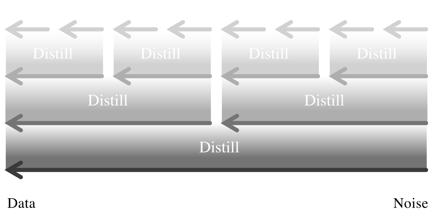
We first introduce the distillation operation of PD in Section 1.3.1, and then summarize the entire training pipeline in Section 1.3.2. Section 1.3.4 presents an extension for CFG guidance.

Distillation Operation in PD

In this section, we fix DDIM in the \({\mathbf{x}}\)-prediction parameterization as the time–stepping rule and still write \(\mathtt{Solver}_{s \to t}\) for the deterministic map obtained by plugging the current teacher’s \({\mathbf{x}}\)-denoiser into DDIM.

In the first PD round (teacher = pre–trained diffusion model), this coincides with integrating the diffusion PF–ODE via DDIM; in later rounds (teacher = previous student), \(\mathtt{Solver}_{s \to t}\) is simply the DDIM transition induced by the current teacher, not the original diffusion PF–ODE.

The distillation step is as follows: starting from a noisy input \({\mathbf{x}}_s\) (a perturbed version of clean data, \({\mathbf{x}}_s = \alpha_s {\mathbf{x}}_0 + \sigma_s \bm{\epsilon}\)), the student is trained to predict a target \({\color{orange}\tilde{\mathbf{x}}}\) so that a single student step \(s\!\to\! t\) reproduces the teacher’s two consecutive steps \(s\!\to\! u\!\to\! t\). Let \({\mathbf{x}}_{\bm{\phi}^\times}({\mathbf{x}},\tau)\) denote the teacher’s \({\mathbf{x}}\)-prediction denoiser in this round. Applying the teacher–induced DDIM transition twice gives \[\tilde{\mathbf{x}}_u := \mathtt{Solver}_{s\to u}\!\left({\mathbf{x}}_s;\,{\mathbf{x}}_{\bm{\phi}^\times}\right), \qquad \tilde{\mathbf{x}}_t := \mathtt{Solver}_{u\to t}\!\left(\tilde{\mathbf{x}}_u;\,{\mathbf{x}}_{\bm{\phi}^\times}\right).\] Here, we use the notation of Equation \(\eqref{eq:solver}\) to denote the deterministic transition map from \(s\) to \(t\) (starting at \({\mathbf{x}}_s\)) induced by plugging \({\mathbf{x}}_{\bm{\phi}^\times}\) into DDIM.

Once a closed-form expression for \({\color{orange}\tilde{\mathbf{x}}}\) is obtained, we train a student model \({\mathbf{f}}_{\bm{\theta}}({\mathbf{x}}_s, s)\) (also an \({\mathbf{x}}\)-prediction model here) to approximate the “two-steps-in-one” target \({\color{orange}\tilde{\mathbf{x}}}\) by minimizing \[\begin{align} \label{eq:pd-optimization} \min_{\bm{\theta}} \mathbb{E}_s \mathbb{E}_{{\mathbf{x}}_s\sim p_s}\!\left[w(\lambda_s)\,\big\|{\mathbf{f}}_{\bm{\theta}}({\mathbf{x}}_s, s) - {\color{orange}\tilde{\mathbf{x}}}\big\|_2^2\right]. \end{align}\]

In the following, we show that the DDIM rule yields \({\color{orange}\tilde{\mathbf{x}}}\) in closed form through elementary algebra (note that the result holds for both discrete and continuous time):

With this formula, PD computes the pseudo-clean target at time \(s\) whose single DDIM step \(s\!\to\!t\) lands exactly at the two-step output \(\tilde{\mathbf{x}}_t\).

Practical Discrete Time Grids and Loss.

In practice, we fix a decreasing grid \(t_0=T>t_1>\cdots>t_N=0\) and, for brevity, write \(s:=t_k\), \(u:=t_{k+1}\), \(t:=t_{k+2}\). The teacher provides one step maps \(\mathtt{Teacher}_{t_k\to t_{k+1}}\), and the student learns a two step skip map that matches the teacher composition: \[\mathtt{Student}_{t_k\to t_{k+2}} \approx \mathtt{Teacher}_{t_{k+1}\to t_{k+2}} \circ \mathtt{Teacher}_{t_{k}\to t_{k+1}}.\]

For the standard halving schedule, assume \(N\) is even and sample triplets \((s,u,t)=(t_k,t_{k+1},t_{k+2})\) with \(k\in\{0,2,\ldots,N-2\}\). The objective Equation \(\eqref{eq:pd-optimization}\) becomes \[\min_{\bm{\theta}} \mathbb{E}_{\,k \sim \mathcal{U}\{0,2,\ldots,N{-}2\}} \mathbb{E}_{\,{\mathbf{x}}_{t_k}\sim p_{t_k}}\! \Big[ w(\lambda_{t_k})\, \big\| {\mathbf{f}}_{\bm{\theta}}({\mathbf{x}}_{t_k},t_k) - {\color{orange}\tilde{\mathbf{x}}}^{(k)} \big\|_2^2 \Big],\] where the teacher two-step target \({\color{orange}\tilde{\mathbf{x}}}^{(k)}\) is computed via Lemma: Two-Steps-in-One Target orange of DDIM. If the grid is uniform, one may write \(t_k = T(1 - k/N)\) so that \[s = T\Big(1 - \frac{k}{N}\Big),\quad u = T\Big(1 - \frac{k+1}{N}\Big),\quad t = T\Big(1 - \frac{k+2}{N}\Big),\] corresponding to evenly spaced time steps of size \(\Delta s = T/N\).

Entire Training Pipeline of PD and Its Sampling

After training on locally paired fragments via Equation \(\eqref{eq:pd-optimization}\), the \(\mathtt{Student}\) no longer follows every interval of the original grid. Instead, each learned step covers two consecutive \(\mathtt{Teacher}\) steps, so the \(\mathtt{Student}\) advances on every other time point, \[t_0 \to t_2 \to t_4 \to \cdots \to t_N,\] and thus traverses the same horizon \([0,T]\) using only \(N/2\) transitions. After this stage, the trained \(\mathtt{Student}\) replaces the \(\mathtt{Teacher}\) as the new denoiser model. The procedure is then repeated on the coarser grid (the time step doubles), yielding the progression \[N \;\to\; N/2 \;\to\; N/4 \;\to\; \cdots,\] until the desired number of inference steps is reached. At each iteration, the new \(\mathtt{Student}\) is initialized from the updated \(\mathtt{Teacher}\). This iterative halving preserves the global time horizon while progressively compressing the temporal resolution of the generative process.

Sampling.

At inference time, using the (DDIM) solver with the current \(\mathtt{Student}\) as the denoiser, the sampler advances on the coarser grid induced by training. After the first round it takes “skip-2” jumps (\(t_0 \to t_2 \to \cdots \to t_N\)), after the next round “skip-4” (\(t_0 \to t_4 \to \cdots \to t_N\)), and so on, halving the number of sampling steps at each iteration while keeping the same start and end times.

Additional Discussion: Local Semigroup Matching and the Possibility of Generalized Solvers

Progressive Distillation as Local Semigroup Matching.

Within the unified objective Equation \(\eqref{eq:general-cm-loss}\), the intractable oracle target \({\bm{\Psi}}_{s\to 0}\) is replaced by a teacher–induced surrogate that uses the semigroup property of the ODE flow (see more details later in Equation in Chapter 11): evolving from \(s\) to \(t\) should be equivalent to going from \(s\) to any intermediate \(u\) and then from \(u\) to \(t\), \[{\bm{\Psi}}_{s\to t} = {\bm{\Psi}}_{u\to t}\circ{\bm{\Psi}}_{s\to u}.\] PD enforces this locally by training the student’s one–step map to match the teacher’s composition of two adjacent one–step fragments: \[\begin{align} \label{eq:pd-local} \mathbb{E}_{s}\mathbb{E}_{{\mathbf{x}}_s\sim p_s} \big\| \underbrace{{\mathbf{G}}_{{\bm{\theta}}}({\mathbf{x}}_s, s, s-2\Delta s)}_{\text{student one-step}} - \underbrace{\mathtt{Solver}_{s-\Delta s\to s-2\Delta s}\big(\mathtt{Solver}_{s\to s-\Delta s}({\mathbf{x}}_s)\big)}_{\text{teacher two-step composition}} \big\|_2^2. \end{align}\] When the teacher solver accurately approximates the underlying ODE flow, the composition in Equation \(\eqref{eq:pd-local}\) approximates the corresponding semigroup relation on a short decreasing grid (take \(s>u>t\) with \(u=s-\Delta s\) and \(t=s-2\Delta s\)): \[\begin{align*} {\bm{\Psi}}_{s\to s-2\Delta s} &= {\bm{\Psi}}_{s-\Delta s\to s-2\Delta s}\circ{\bm{\Psi}}_{s\to s-\Delta s} \\&\approx \mathtt{Solver}_{s-\Delta s\to s-2\Delta s}\circ \mathtt{Solver}_{s\to s-\Delta s}, \end{align*}\] so training only requires short teacher fragments, rather than a full rollout from time \(s\) all the way to \(0\).

To connect back to the few–step denoiser view in Equation \(\eqref{eq:general-cm-loss}\), define the student’s few–step map as a composition of learned jumps: \[\underbrace{{\mathbf{G}}_{{\bm{\theta}}}({\mathbf{x}}_s, s, 0)}_{\text{few-step denoiser}} = \big({\mathbf{G}}_{{\bm{\theta}}}(\,\cdot\,, 2\Delta s, 0)\circ\cdots\circ {\mathbf{G}}_{{\bm{\theta}}}(\,\cdot\,, s, s-2\Delta s)\big)({\mathbf{x}}_s).\] Conceptually, Equation \(\eqref{eq:pd-local}\) provides an efficient local surrogate for the global regression \[\mathbb{E}_{s,{\mathbf{x}}_s}\Big\|{\mathbf{G}}_{{\bm{\theta}}}({\mathbf{x}}_s,s,0)\;-\;(\mathtt{Solver})^{\circ}_{s\to 0}({\mathbf{x}}_s)\Big\|_2^2,\] where \((\mathtt{Solver})^{\circ}_{s\to 0}\) denotes the teacher’s full composition from \(s\) to \(0\) on a grid with step size \(\Delta s\), serving as a proxy for \({\bm{\Psi}}_{s\to 0}\).

Can we Use Other Solvers?

Above, we used DDIM in the \({\mathbf{x}}\)-prediction parameterization as a concrete PF–ODE sampler. The basic distillation principle is more general: several fine teacher steps produce a target endpoint, and the student is trained so that one coarser step reaches the same endpoint.

The closed-form pseudo-target derived above is available whenever the coarse solver update can be inverted with respect to the student’s network prediction. For DDIM, the update is affine in a single \({\mathbf{x}}\)-prediction, so this inversion is analytic. The same idea applies to other solvers whose one-step update admits a comparable inversion.

For more complicated solvers, such a single-output inversion may not be available. Multi-stage methods use several network evaluations, multi-step methods depend on previous solver states, and implicit methods require solving coupled equations. In such cases, one can instead compute the endpoint of the coarse student step and directly match it to the endpoint produced by the fine teacher steps, as in Equation \(\eqref{eq:pd-local}\), backpropagating through the student solver when feasible. Since a coarse step may itself require multiple neural function evaluations, fewer time steps do not necessarily imply the same reduction in NFE.

For a stochastic sampler, the same pathwise logic applies after fixing or coupling the random draws used by the teacher and student. Without such coupling, individual trajectories need not share the same endpoint, and the appropriate target is generally distributional rather than pathwise matching.

PD with Guidance

Meng et al. (2023) proposed a two-stage pipeline for distilling classifier-free guided (CFG) diffusion models: (1) distill the guidance into a single network that takes the guidance weight as input, and (2) apply progressive distillation (PD) to reduce the sampling steps. They demonstrated this both in pixel space and in latent space (e.g., Stable Diffusion).

Stage-One Distillation: Distilling Guidance.

Let \({\mathbf{x}}_{\bm{\phi}^\times}({\mathbf{x}}_s, s, {\mathbf{c}})\) denote the (pre-trained) conditional diffusion model output in the “\({\mathbf{x}}\)-prediction” parameterization (i.e., a clean estimate) at time \(s\) and condition \({\mathbf{c}}\); the condition can also be null, \({\mathbf{c}}=\emptyset\) (unconditional branch). The \(\omega\)-weighted CFG combination in Equation in Chapter 8 can be written as \[\begin{equation} \label{eq:cfg-model-clean} {\mathbf{x}}_{\bm{\phi}^\times}^{\,\omega}({\mathbf{x}}_s, s, {\mathbf{c}}) := (1+\omega)\,{\mathbf{x}}_{\bm{\phi}^\times}({\mathbf{x}}_s, s, {\mathbf{c}}) - \omega\,{\mathbf{x}}_{\bm{\phi}^\times}({\mathbf{x}}_s, s, \emptyset), \end{equation}\] where \(\omega \sim p_\omega(\omega)\) for some CFG weighting distribution \(p_\omega\), typically \(p_\omega(\omega)=\mathcal{U}[\omega_{\min},\omega_{\max}]\).

Stage-one introduces a new model \({\mathbf{x}}_{\bm{\theta}_1}({\mathbf{x}}_s, s, {\mathbf{c}}, \omega)\) that directly takes \(\omega\) as input and learns to reproduce the CFG output \({\mathbf{x}}_{\bm{\phi}^\times}^{\,\omega}({\mathbf{x}}_s, s, {\mathbf{c}})\) by supervised regression: \[\min_{\bm{\theta}_1}\; \mathbb{E}_{\omega\sim p_\omega, s, {\mathbf{x}}\sim p_{\mathrm{data}}, {\mathbf{x}}_s \sim p({\mathbf{x}}_s\mid {\mathbf{x}})} \lambda(s) \big\|{\mathbf{x}}_{\bm{\theta}_1}({\mathbf{x}}_s, s, {\mathbf{c}}, \omega)-{\mathbf{x}}_{\bm{\phi}^\times}^{\omega}({\mathbf{x}}_s, s, {\mathbf{c}})\big\|_2^2.\] Here \(\lambda(s)\) is a standard schedule-dependent weighting; sampling \(\omega\) each iteration teaches a single network to emulate CFG at arbitrary guidance strengths.

Stage-Two Distillation: PD.

The stage-one model \({\mathbf{x}}_{\bm{\theta}_1}({\mathbf{x}}_s, s, {\mathbf{c}}, \omega)\) serves as the teacher in PD and is progressively distilled into a student \({\mathbf{x}}_{\bm{\theta}_2}({\mathbf{x}}_s, s, {\mathbf{c}}, \omega)\) with fewer sampling steps, following Section 1.3.2. At each iteration, the number of steps is halved (e.g., \(N \to N/2 \to N/4 \to \cdots\)).

Closing Remarks

This chapter has introduced our first major paradigm for training-based acceleration. Having exhausted training-free improvements via numerical solvers, we shifted our focus to a new strategy: training a fast student generator that learns to replicate the behavior of a slow, pre-trained teacher diffusion model.

We explored two primary distillation philosophies. First, in distribution-based distillation, represented by methods like Variational Score Distillation (VSD), the student’s output distribution is trained to match the teacher’s. This is achieved by aligning their respective score functions across different noise levels, providing a stable, non-adversarial objective. Second, in flow map distillation, we saw how methods like Progressive Distillation (PD) train the student to directly approximate the teacher’s solution trajectory. PD’s iterative approach, where each round halves the number of sampling steps, proved to be a powerful and practical method for compressing a long iterative process into just a few steps.

These distillation techniques successfully bridge the gap between the high sample quality of iterative diffusion models and the inference speed of one-step generators, offering a compelling pathway to efficient, high-fidelity synthesis.

However, the reliance on a pre-trained teacher model introduces a two-stage pipeline: first train a slow but powerful teacher, then distill it into a fast student. This raises a fundamental question at the forefront of generative modeling research: Can we bypass the teacher entirely?

Is it possible to design a standalone training principle that learns these fast, few-step generators directly from data? The final chapter of this monograph will address this question.

1. We will explore pioneering methods such as Consistency Models that learn the mapping from any point on an ODE trajectory to its destination point.

2. We will delve into generalized concepts of Consistency Models which learn to map any point on an ODE trajectory to another point in a single step.

This shift from improving the solver or distilling a solution to learning the solution map itself represents a significant step toward a new class of generative models that are both principled and highly efficient by design.