Chapter 1: Deep Generative Modeling
What I cannot create, I do not understand.
Richard P. Feynman
Deep generative models (DGMs) are neural networks that learn a probability distribution over high-dimensional data (e.g., images, text, audio) so they can generate new examples that resemble the dataset. We denote the model distribution by \(p_{{\bm{\phi}}}\) and the data distribution by \(p_{\mathrm{data}}\). Given a finite dataset, we fit \({\bm{\phi}}\) by minimizing a loss that measures how far \(p_{{\bm{\phi}}}\) is from \(p_{\mathrm{data}}\). After training, generation amounts to running the model’s sampling procedure to draw \({\mathbf{x}}\sim p_{{\bm{\phi}}}\) (the density \(p_{{\bm{\phi}}}({\mathbf{x}})\) may or may not be directly computable, depending on the model class). Model quality is judged by how well generated samples and their summary statistics match those of \(p_{\mathrm{data}}\), together with task-specific or perceptual metrics.
This chapter builds the mathematical and conceptual foundations behind these ideas. We formalize the problem in Section 1.1, present representative model classes in Section 1.2, and summarize a practical taxonomy in Section 1.3.
After this chapter, you will be able to...
explain, in plain language, what a generative model is trying to learn from a dataset and what it means to model the data distribution;
understand the core idea behind autoregressive models, VAEs, energy-based models, normalizing flows, GANs, and diffusion models, and see how they differ in the way they learn and generate new samples;
Reader route. If you are already familiar with the basic ideas behind modern generative models, you may skim this chapter and use it later as a quick reference.
What is Deep Generative Modeling?
DGMs take as input a large collection of real-world examples (e.g., images, text) drawn from an unknown and complex distribution \(p_{\mathrm{data}}\) and output a trained neural network that parameterizes an approximate distribution \(p_{{\bm{\phi}}}\). Their goals are twofold:
Realistic Generation: To generate novel, realistic samples indistinguishable from real data.
Controllable Generation: To enable fine-grained and interpretable control over the generative process.
This section presents the fundamental concepts and motivations behind DGMs, preparing for a detailed exploration of their mathematical framework and practical applications.
Mathematical Setup
Suppose we are given a finite collection of examples \(\{{\mathbf{x}}^{(i)}\}_{i=1}^N\), such as images, audio, or text. We imagine that these examples were drawn from some underlying data distribution \(p_{\mathrm{data}}\), but we do not know this distribution explicitly. In particular, we only observe the available training examples; we do not have a formula for \(p_{\mathrm{data}}\) or a direct procedure for drawing arbitrary new samples from it1.
Goal of DGM.
The goal of deep generative modeling is therefore to learn a model that can produce new samples whose statistical characteristics resemble those of the observed data. We denote the distribution represented by a model with parameters \(\bm{\phi}\) by \(p_{\bm{\phi}}\). After training, we denote the learned parameters by \(\bm{\phi}^{\times}\) and hope that, in the aspects relevant to generation, \[p_{\bm{\phi}^{\times}} \approx p_{\mathrm{data}}.\] This expression should be understood conceptually: with finite data, finite model capacity, and imperfect optimization, we do not expect the two distributions to be exactly identical. Rather, the learned model should capture enough of the structure of the data distribution to generate realistic and diverse new examples.
Once the model is trained, generation simply means drawing a new sample \[{\mathbf{x}}\sim p_{\bm{\phi}^{\times}}.\] Different families of generative models provide different mechanisms for doing this. Some models additionally allow us to evaluate how much density they assign to an observed sample, while others are primarily defined through their sampling procedure. This distinction will become useful later when we discuss how different generative models are trained; for now, the central objective is simply to learn a distribution from data from which we can generate new samples.
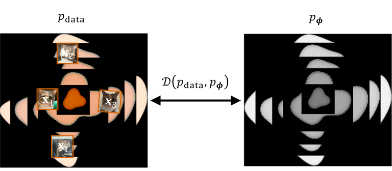
Training of DGM.
We learn parameters \(\bm{\phi}\) of a model family \(\{p_{\bm{\phi}}\}\) by minimizing a discrepancy \(\mathcal{D}(p_{\mathrm{data}},p_{\bm{\phi}})\): \[\begin{align} \label{eq:dgm-optimization} \bm{\phi}^\ast \in \arg\min_{\bm{\phi}}\; \mathcal{D}(p_{\mathrm{data}},p_{\bm{\phi}}). \end{align}\] Because \(p_{\mathrm{data}}\) is unknown, a practical choice of \(\mathcal{D}\) must admit efficient estimation from i.i.d. samples from \(p_{\mathrm{data}}\). With sufficient capacity, \(p_{\bm{\phi}^\ast}\) can closely approximate \(p_{\mathrm{data}}\).
Forward KL and Maximum Likelihood Estimation (MLE).
How should we choose the model parameters so that \(p_{\bm{\phi}}\) resembles \(p_{\mathrm{data}}\)? When the model density \(p_{\bm{\phi}}({\mathbf{x}})\) can be evaluated, a natural idea is to make the observed data receive high density under the model. This leads to maximum likelihood estimation (MLE): we choose \(\bm{\phi}\) so that the training examples are collectively assigned high model density2.
A standard way to formalize this idea is through the (forward) Kullback–Leibler divergence3 \[\begin{align*} \mathcal{D}_{\mathrm{KL}} \big(p_{\mathrm{data}}\|p_{\bm{\phi}}\big) :=\;& \int p_{\mathrm{data}}({\mathbf{x}}) \log \frac{p_{\mathrm{data}}({\mathbf{x}})} {p_{\bm{\phi}}({\mathbf{x}})} \,\mathop{}\!\mathrm{d}{\mathbf{x}} \\ =\;& \mathbb{E}_{{\mathbf{x}}\sim p_{\mathrm{data}}} \big[ \log p_{\mathrm{data}}({\mathbf{x}}) - \log p_{\bm{\phi}}({\mathbf{x}}) \big]. \end{align*}\] The KL divergence is asymmetric, i.e., \[\mathcal{D}_{\mathrm{KL}} \big(p_{\mathrm{data}}\|p_{\bm{\phi}}\big) \neq \mathcal{D}_{\mathrm{KL}} \big(p_{\bm{\phi}}\|p_{\mathrm{data}}\big).\]
At first, the forward KL may appear unusable because the data density \(p_{\mathrm{data}}({\mathbf{x}})\) is unknown. However, it can be decomposed as \[\begin{align*} \mathcal{D}_{\mathrm{KL}} \big(p_{\mathrm{data}}\|p_{\bm{\phi}}\big) = \mathbb{E}_{{\mathbf{x}}\sim p_{\mathrm{data}}} \left[ \log \frac{p_{\mathrm{data}}({\mathbf{x}})} {p_{\bm{\phi}}({\mathbf{x}})} \right] = -\mathbb{E}_{{\mathbf{x}}\sim p_{\mathrm{data}}} \big[ \log p_{\bm{\phi}}({\mathbf{x}}) \big] - \mathcal{H}\big(p_{\mathrm{data}}\big), \end{align*}\] where \[\mathcal{H}\big(p_{\mathrm{data}}\big) := -\mathbb{E}_{{\mathbf{x}}\sim p_{\mathrm{data}}} \big[ \log p_{\mathrm{data}}({\mathbf{x}}) \big]\] is the entropy of the data distribution. Crucially, this term does not depend on \(\bm{\phi}\). Therefore, although we cannot evaluate \(p_{\mathrm{data}}({\mathbf{x}})\) itself, we do not need to know it in order to optimize the model parameters. This gives the following equivalence:
Lemma: Minimizing KL \(\Leftrightarrow\) MLE
\[\begin{align} \label{eq:MLE} \min_{\bm{\phi}}\, \mathcal{D}_{\mathrm{KL}} \big( p_{\mathrm{data}} \,\|\, p_{\bm{\phi}} \big) \;\Longleftrightarrow\; \max_{\bm{\phi}}\, \mathbb{E}_{{\mathbf{x}}\sim p_{\mathrm{data}}} \big[ \log p_{\bm{\phi}}({\mathbf{x}}) \big]. \end{align}\]
In words, minimizing the forward KL divergence is equivalent to making real data samples receive high log-likelihood under the model. This is exactly maximum likelihood estimation.
In practice, the expectation over \(p_{\mathrm{data}}\) is replaced by the available training samples \(\{{\mathbf{x}}^{(i)}\}_{i=1}^{N}\), assumed to be drawn i.i.d. from \(p_{\mathrm{data}}\). This gives the empirical negative log-likelihood objective \[\begin{align*} \hat{\mathcal{L}}_{\mathrm{MLE}}(\bm{\phi}) := -\frac{1}{N} \sum_{i=1}^{N} \log p_{\bm{\phi}}\big({\mathbf{x}}^{(i)}\big), \end{align*}\] which can be optimized using stochastic gradients over minibatches. Thus, MLE requires only samples from \(p_{\mathrm{data}}\); it does not require evaluating the unknown data density itself.
The direction of the KL divergence matters because it determines where the discrepancy is averaged. For the forward KL, \[\mathcal{D}_{\mathrm{KL}} \big(p_{\mathrm{data}}\|p_{\bm{\phi}}\big) = \mathbb{E}_{{\mathbf{x}}\sim p_{\mathrm{data}}} \left[ \log \frac{p_{\mathrm{data}}({\mathbf{x}})} {p_{\bm{\phi}}({\mathbf{x}})} \right],\] the expectation is taken over the data distribution. Thus, regions that occur under \(p_{\mathrm{data}}\) must be accounted for by the model. By contrast, the reverse KL, \(\mathcal{D}_{\mathrm{KL}} (p_{\bm{\phi}}\|p_{\mathrm{data}})\), averages instead over samples from the model distribution.
This difference has an important consequence. Suppose there exists a region \(A\) with positive data probability, \(p_{\mathrm{data}}(A)>0\), but the model assigns zero density there, \(p_{\bm{\phi}}({\mathbf{x}})=0\) for \({\mathbf{x}}\in A\). Then the forward KL becomes infinite, since \[\log \frac{p_{\mathrm{data}}({\mathbf{x}})} {p_{\bm{\phi}}({\mathbf{x}})} = +\infty\] on that region. Therefore, minimizing the forward KL strongly penalizes a model for completely missing regions where the data distribution places probability mass. This behavior is commonly referred to as mode covering.
Fisher Divergence.
The Fisher divergence is another important concept for (score-based) diffusion modeling (see Chapter 3). For two distributions \(p\) and \(q\), it is defined as \[\begin{align} \label{eq:fisher} \mathcal D_{\mathrm F}(p \| q) := \mathbb{E}_{\mathbf{x}\sim p} \left[ \left\|\nabla_{\mathbf x}\log p(\mathbf x)-\nabla_{\mathbf x}\log q(\mathbf x)\right\|_2^{2} \right]. \end{align}\] It measures the discrepancy between the score functions \(\nabla_{\mathbf x}\log p(\mathbf x)\) and \(\nabla_{\mathbf x}\log q(\mathbf x)\), which are vector fields pointing toward regions of higher probability. In short, \(\mathcal D_{\mathrm F}(p \| q)\ge 0\) with equality if and only if \(p=q\) almost everywhere. It is invariant to normalization constants, since scores depend only on gradients of log-densities, and it forms the basis of score matching (Equation in Chapter 3 and Equation in Chapter 3): a method that learns the gradient of the log-density for generation (score-based models). In this setting, the data distribution \(p=p_{\mathrm{data}}\) serves as the target, while the model \(q=p_{\bm{\phi}}\) is trained to align its score field with that of the data.
Beyond KL.
Although the KL divergence is the most widely used measure of difference between probability distributions, it is not the only one. Different divergences capture different geometric or statistical notions of discrepancy, which in turn affect the optimization dynamics of learning algorithms. A broad family is the \(f\)-divergences (Csiszár 1963): \[\begin{align} \label{eq:f-div} \mathcal{D}_f(p\|q) =\int q({\mathbf{x}}) f \left(\frac{p({\mathbf{x}})}{q({\mathbf{x}})}\right)\mathop{}\!\mathrm{d}{\mathbf{x}}, \qquad f(1)=0, \end{align}\] where \(f:\mathbb{R}_+ \to\mathbb{R}\) is a convex function. By changing \(f\), we obtain many well-known divergences: \[\begin{aligned} f(u)&=u\log u &&\Rightarrow&& \mathcal{D}_f=\mathcal{D}_{\mathrm{KL}}(p\|q)\quad\text{(forward KL)},\\ f(u)&=\tfrac12 \left[u\log u-(u+1)\log \tfrac{1+u}{2}\right] &&\Rightarrow&& \mathcal{D}_f=\mathcal{D}_{\mathrm{JS}}(p\|q)\quad\text{(Jensen--Shannon)},\\ f(u)&=\tfrac12|u-1| &&\Rightarrow&& \mathcal{D}_f=\mathcal{D}_{\mathrm{TV}}(p,q)\quad\text{(total variation)}. \end{aligned}\] For clarity, the explicit forms are \[\mathcal{D}_{\mathrm{JS}}(p\|q)=\tfrac12 \mathcal{D}_{\mathrm{KL}}\big(p\| \tfrac12(p+q)\big)+\tfrac12 \mathcal{D}_{\mathrm{KL}}\big(q\| \tfrac12(p+q)\big),\] and \[\mathcal{D}_{\mathrm{TV}}(p,q)=\tfrac12 \int_{\mathbb{R}^D } |p-q|\mathop{}\!\mathrm{d}{\mathbf{x}} =\sup_{A\subset \mathbb{R}^D } |p(A)-q(A)|.\] Intuitively, the JS divergence provides a smooth and symmetric measure that balances both distributions and avoids the unbounded penalties of KL (we will later see that it helps interpret the Generative Adversarial Network (GAN) framework), while the total variation distance captures the largest possible probability difference between the two.
A different viewpoint comes from optimal transport (see Chapter 7), whose representative is the Wasserstein distance (see eq: Monge's Formulation). It measures the minimal cost of moving probability mass from one distribution to another. Unlike \(f\)-divergences, which compare density ratios, Wasserstein distances depend on the geometry of the sample space and remain meaningful even when the supports of \(p\) and \(q\) do not overlap.
Each divergence embodies a different notion of closeness between distributions and thus induces distinct learning behavior. We will revisit these divergences when they arise naturally in the context of generative modeling throughout this monograph.
Challenges in Modeling Distributions
To model a complex data distribution, we can parameterize the probability density function \(p_{\mathrm{data}}\) using a neural network with parameters \(\bm{\phi}\), creating a model we denote as \(p_{\bm{\phi}}\). For \(p_{\bm{\phi}}\) to be a valid probability density function, it must satisfy two fundamental properties:
Non-Negativity: \(p_{\bm{\phi}}({\mathbf{x}}) \ge 0\) for all \({\mathbf{x}}\) in the domain.
Normalization: The integral over the entire domain must equal one, i.e., \(\int p_{\bm{\phi}}({\mathbf{x}}) \mathop{}\!\mathrm{d}{\mathbf{x}}= 1\).
A network can naturally produce a real scalar \(E_{{\bm{\phi}}}({\mathbf{x}}) \in \mathbb{R}\) for input \({\mathbf{x}}\). To interpret this output as a valid density, it must be transformed to satisfy conditions (i) and (ii). A practical alternative is to view \(E_{{\bm{\phi}}}\colon\mathbb{R}^D\to\mathbb{R}\) as defining an unnormalized density and then enforce these properties explicitly.
Step 1: Ensuring Non-Negativity.
We can guarantee that our model’s output is always non-negative by applying a positive function to the raw output of the neural network \(E_{\bm{\phi}}({\mathbf{x}})\), such as \(\left|E_{\bm{\phi}}({\mathbf{x}})\right|\), \(E^2_{\bm{\phi}}({\mathbf{x}})\). A standard and convenient choice is the exponential function. This gives us an unnormalized density, \(\tilde{p}_{\bm{\phi}}({\mathbf{x}})\), that is guaranteed to be positive: \[\tilde{p}_{\bm{\phi}}({\mathbf{x}}) = \exp(E_{\bm{\phi}}({\mathbf{x}})).\]
Step 2: Enforcing Normalization.
The function \(\tilde{p}_{\bm{\phi}}({\mathbf{x}})\) is positive but does not integrate to one. To create a valid probability density, we must divide it by its integral over the entire space. This leads to the final form of our model: \[p_{\bm{\phi}}({\mathbf{x}}) = \frac{\tilde{p}_{\bm{\phi}}({\mathbf{x}})}{\int \tilde{p}_{\bm{\phi}}({\mathbf{x}}') \mathop{}\!\mathrm{d}{\mathbf{x}}'} = \frac{\exp(E_{\bm{\phi}}({\mathbf{x}}))}{\int \exp(E_{\bm{\phi}}({\mathbf{x}}')) \mathop{}\!\mathrm{d}{\mathbf{x}}'}.\] The denominator in this expression is known as the normalizing constant or partition function, denoted by \(Z(\bm{\phi})\): \[Z(\bm{\phi}) := \int \exp(E_{\bm{\phi}}({\mathbf{x}}')) \mathop{}\!\mathrm{d}{\mathbf{x}}'.\] While this procedure provides a valid construction for \(p_{\bm{\phi}}({\mathbf{x}})\), it introduces a major computational challenge. For most high-dimensional problems, the integral required to compute the normalizing constant \(Z(\bm{\phi})\) is intractable. This intractability is a central problem that motivates the development of many different families of deep generative models.
In the following sections, we introduce several prominent approaches of DGM. Each is designed to circumvent or reduce the computational cost of evaluating this normalizing constant.
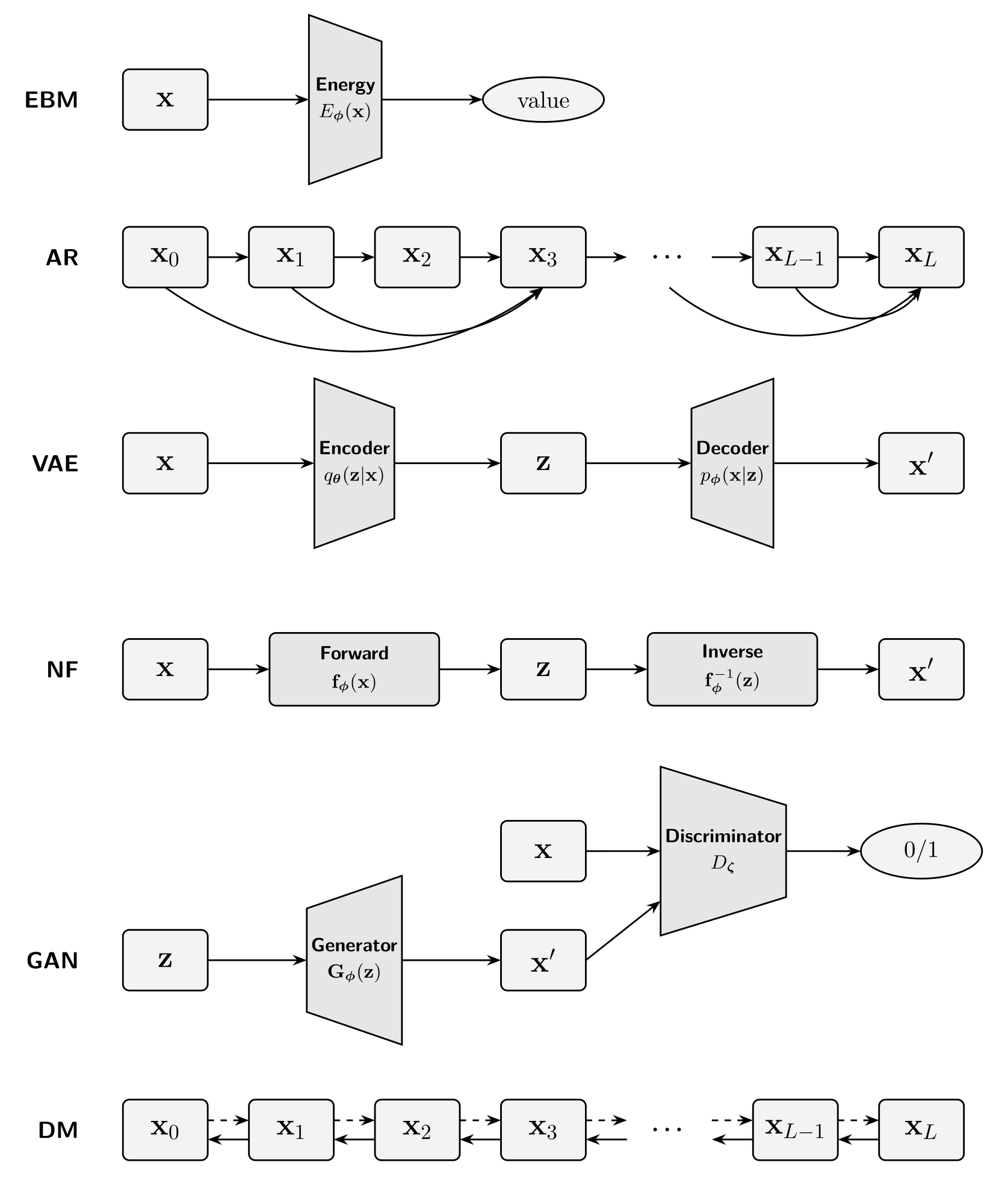
Prominent Deep Generative Models
A central challenge in generative modeling is to learn expressive probabilistic models that can capture the rich and complex structure of high-dimensional data. Over the years, various modeling strategies have been developed, each making different trade-offs between tractability, expressiveness, and training efficiency. In this section, we explore some of the most influential strategies that have shaped the field, accompanied by a comparison of their computation graphs in Figure 1.2.
Energy-Based Models (EBMs).
EBMs (Ackley et al. 1985; LeCun et al. 2006) define a probability distribution through an energy function \(E_{\bm{\phi}}({\mathbf{x}})\) that assigns lower energy to more probable data points. The probability of a data point is defined as: \[\begin{equation*} p_{\bm{\phi}}({\mathbf{x}}) := \frac{1}{Z({\bm{\phi}})} \exp(-E_{\bm{\phi}}({\mathbf{x}})), \end{equation*}\] where \[Z({\bm{\phi}}) = \int \exp(-E_{\bm{\phi}}({\mathbf{x}})) \mathop{}\!\mathrm{d}{\mathbf{x}}\] is the partition function. Training EBMs typically involves maximizing the log-likelihood of the data. However, this requires techniques to address the computational challenges arising from the intractability of the partition function. In the following chapter, we will explore how Diffusion Models offer an alternative by generating data from the gradient of the log density, which does not depend on the normalizing constant, thereby circumventing the need for partition function computation.
Autoregressive Models.
Deep autoregressive (AR) models (Frey et al. 1995; Larochelle and Murray 2011; Uria et al. 2016) build on a simple but powerful observation: any joint distribution can be decomposed into a sequence of conditional distributions using the chain rule of probability. For a chosen ordering of the variables \(\mathbf{x}=(x_1,\ldots,x_D)\), the data distribution satisfies \[\begin{equation*} p_{\mathrm{data}}(\mathbf{x}) = \prod_{i=1}^{D} p_{\mathrm{data}}(x_i | \mathbf{x}_{<i}), \qquad \mathbf{x}_{<i}=(x_1,\ldots,x_{i-1}). \end{equation*}\] Importantly, this factorization is an exact identity rather than a modeling assumption: any joint distribution admits such a decomposition for any chosen ordering of its variables.
The challenge is that the true conditional distributions \(p_{\mathrm{data}}(x_i|\mathbf{x}_{<i})\) are unknown. AR models therefore parameterize a model with the same factorized form, \[\begin{equation*} p_{\bm{\phi}}(\mathbf{x}) = \prod_{i=1}^{D} p_{\bm{\phi}}(x_i|\mathbf{x}_{<i}), \end{equation*}\] and use a neural network, such as a Transformer, to approximate these conditional distributions from data. For example, for discrete data the network may output a categorical distribution through a softmax, whereas for continuous data it may output the parameters of a tractable conditional density. Because every conditional distribution is normalized, their product automatically defines a normalized joint distribution.
This construction also makes likelihood-based training particularly simple. For a data sample \(\mathbf{x}\), the log-likelihood decomposes as \[\begin{equation*} \log p_{\bm{\phi}}(\mathbf{x}) = \sum_{i=1}^{D} \log p_{\bm{\phi}}(x_i|\mathbf{x}_{<i}), \end{equation*}\] so the model can be trained directly by maximum likelihood, or equivalently by minimizing the negative log-likelihood. During training, the observed preceding variables \(\mathbf{x}_{<i}\) are available, so many of these conditional predictions can typically be evaluated in parallel.
Generation, however, remains inherently sequential: \[\begin{equation*} x_1 \sim p_{\bm{\phi}}(x_1), \qquad x_2 \sim p_{\bm{\phi}}(x_2| x_1), \qquad \ldots, \qquad x_D \sim p_{\bm{\phi}}(x_D|\mathbf{x}_{<D}). \end{equation*}\] Thus, AR models provide tractable exact likelihoods and flexible density modeling, but sampling requires generating variables one after another and can therefore become computationally expensive for long sequences. AR models remain a foundational class of likelihood-based generative models and underlie many modern sequence and language models.
Variational Autoencoders (VAEs).
VAEs (Kingma and Welling 2013) extend classical autoencoders by introducing latent variables \({\mathbf{z}}\) that capture hidden structure in the data \({\mathbf{x}}\). Instead of directly learning a mapping between \({\mathbf{x}}\) and \({\mathbf{z}}\), VAEs adopt a probabilistic view: they learn both an encoder, \(q_{{\bm{\theta}}}({\mathbf{z}}|{\mathbf{x}})\), which approximates the unknown distribution of latent variables given the data, and a decoder, \(p_{{\bm{\phi}}}({\mathbf{x}}|{\mathbf{z}})\), which reconstructs data from these latent variables. To make training feasible, VAEs maximize a tractable surrogate to the true log-likelihood, called the Evidence Lower Bound (ELBO): \[\begin{equation*} \mathcal{L}_{\text{ELBO}}({\bm{\theta}}, {\bm{\phi}}; {\mathbf{x}}) = \mathbb{E}_{q_{{\bm{\theta}}}({\mathbf{z}}| {\mathbf{x}})} \left[ \log p_{{\bm{\phi}}}({\mathbf{x}}| {\mathbf{z}}) \right] - \mathcal D_{\mathrm{KL}} \left( q_{{\bm{\theta}}}({\mathbf{z}}| {\mathbf{x}}) \,\|\, p_{\mathrm{prior}}({\mathbf{z}}) \right). \end{equation*}\] Here, the first term encourages accurate reconstruction of the data, while the second regularizes the latent variables by keeping them close to a simple prior distribution \(p_{\mathrm{prior}}({\mathbf{z}})\) (often Gaussian).
VAEs provide a principled way to combine neural networks with latent-variable models and remain one of the most widely used likelihood-based approaches. However, they also face practical challenges, such as limited sample sharpness and training pathologies (e.g., the tendency of the decoder to ignore latent variables). Despite these limitations, VAEs laid important foundations for later advances, including diffusion models.
Normalizing Flows.
Classic flow-based generative models include Normalizing Flows (NFs) (Rezende and Mohamed 2015) and their continuous-time counterparts based on Neural Ordinary Differential Equations (NODEs) (Chen et al. 2018), aim to learn a bijective mapping \({\mathbf{f}}_{\bm{\phi}}\) between a simple latent distribution \({\mathbf{z}}\) and a complex data distribution \({\mathbf{x}}\) via an invertible operator. This is achieved either through a sequence of bijective transformations (in NFs) or by modeling the transformation as an Ordinary Differential Equation (in NODEs). These models leverage the “change-of-variable formula for densities”, enabling MLE training: \[\begin{equation*} \log p_{\bm{\phi}}({\mathbf{x}}) = \log p({\mathbf{z}}) + \log \left| \det \frac{\partial {\mathbf{f}}_{\bm{\phi}}^{-1}({\mathbf{x}})}{\partial {\mathbf{x}}} \right|, \end{equation*}\] where \({\mathbf{f}}_{\bm{\phi}}\) represents the invertible transformation mapping \({\mathbf{z}}\) to \({\mathbf{x}}\). NFs explicitly model normalized densities using invertible transformations with tractable Jacobian determinants. The normalization constant is absorbed analytically via the change-of-variables formula, making likelihood computation exact and tractable.
Despite their conceptual elegance, classic flow-based models often face practical limitations. For instance, NFs typically impose restrictive architectural constraints to ensure bijectivity, while NODEs may encounter training inefficiencies due to the computational overhead of solving ODEs. Both approaches face challenges when scaling to high-dimensional data. In later chapters, we will explore how Diffusion Models relate to and build upon these classic flow-based methods.
Generative Adversarial Networks (GANs).
GANs (Goodfellow et al. 2014) consist of two neural networks, a generator \({\mathbf{G}}_{\bm{\phi}}\) and a discriminator \(D_{\bm{\zeta}}\), that compete against each other. The generator aims to create realistic samples \({\mathbf{G}}_{\bm{\phi}}({\mathbf{z}})\) from random noise \({\mathbf{z}}\sim p_{\mathrm{prior}}\), while the discriminator attempts to distinguish between real samples \({\mathbf{x}}\) and generated samples \({\mathbf{G}}_{\bm{\phi}}({\mathbf{z}})\). The objective function for GANs can be formulated as: \[\begin{equation*} \min_{{\mathbf{G}}_{\bm{\phi}}} \max_{D_{\bm{\zeta}}} \underbrace{\mathbb{E}_{{\mathbf{x}}\sim p_{\mathrm{data}}({\mathbf{x}})}[\log D_{\bm{\zeta}}({\mathbf{x}})]}_{\text{real}} + \underbrace{\mathbb{E}_{{\mathbf{z}}\sim p_{\mathrm{prior}}({\mathbf{z}})}\left[\log(1 - D_{\bm{\zeta}}\left({\mathbf{G}}_{\bm{\phi}}({\mathbf{z}}))\right)\right]}_{\text{fake}}. \end{equation*}\] GANs do not define an explicit density function and therefore bypass likelihood estimation entirely. Instead of computing a normalization constant, they focus on generating samples that closely mimic the data distribution.
From a divergence perspective, the discriminator implicitly measures the discrepancy between the true data distribution \(p_{\mathrm{data}}\) and the generator distribution \(p_{{\mathbf{G}}_{{\bm{\phi}}}}\), where \(p_{{\mathbf{G}}_{{\bm{\phi}}}}\) denotes the distribution of generated samples \({\mathbf{G}}_{{\bm{\phi}}}({\mathbf{z}})\) obtained from noise \({\mathbf{z}}\sim p_{\mathrm{prior}}\). With an optimal discriminator for a fixed generator \({\mathbf{G}}_{{\bm{\phi}}}\) computed as \[\begin{equation*} \frac{p_{\mathrm{data}}({\mathbf{x}})}{p_{\mathrm{data}}({\mathbf{x}}) + p_{{\mathbf{G}}_{{\bm{\phi}}}}({\mathbf{x}})}, \end{equation*}\] the generator’s minimization reduces to \[\begin{equation*} \min_{{\mathbf{G}}_{{\bm{\phi}}}} \; 2\,\mathcal{D}_\mathrm{JS} \left(p_{\mathrm{data}} \,\|\, p_{{\mathbf{G}}_{\bm{\phi}}}\right) - \log 4. \end{equation*}\] Here, \(\mathcal{D}_\mathrm{JS}\) denotes the Jensen–Shannon divergence, defined as \[\begin{equation*} \mathcal{D}_\mathrm{JS}(p \,\|\, q) := \tfrac{1}{2} \mathcal{D}_\mathrm{KL} \left(p \,\middle\|\, \tfrac{p+q}{2}\right) + \tfrac{1}{2} \mathcal{D}_\mathrm{KL} \left(q \,\middle\|\, \tfrac{p+q}{2}\right). \end{equation*}\] This shows that GANs implicitly minimize \(\mathcal{D}_\mathrm{JS}(p_{\mathrm{data}} \,\|\, p_{{\mathbf{G}}_{\bm{\phi}}})\). More broadly, extensions such as \(f\)-GANs (Nowozin et al. 2016) generalize this view by demonstrating that adversarial training can minimize a family of \(f\)-divergences, placing GANs within the same divergence-minimization framework as other generative models.
Although GANs are capable of generating high-quality data, their min-max training process is notoriously unstable, often requiring carefully designed architectures and engineering techniques to achieve satisfactory performance. However, GANs have since been revived as an auxiliary component to enhance other generative models, particularly Diffusion Models.
Taxonomy of Modeling
As we have seen, DGMs span a wide spectrum of modeling strategies. A fundamental distinction lies in how these models parameterize the underlying data distribution, that is, whether they specify \(p_{\bm{\phi}}(\mathbf{x})\) explicitly or only implicitly, irrespective of the training objective.
Explicit Models: These models directly parameterize a probability distribution \(p_{\bm{\phi}}(\mathbf{x})\) via a tractable or approximately tractable density or mass function. Examples include ARs, NFs, VAEs, and DMs, all of which define \(p_{\bm{\phi}}(\mathbf{x})\) either exactly or through a tractable bound.
Implicit Models: These models specify a distribution only through a sampling procedure, typically of the form \(\mathbf{x} = {\mathbf{G}}_{\bm{\phi}}(\mathbf{z})\) for some noise variable \(\mathbf{z} \sim p_{\mathrm{prior}}\). In this case, \(p_{\bm{\phi}}(\mathbf{x})\) is not available in closed form and may not be defined at all.
The table in Table 1.1 offers a concise summary of these contrasting approaches.
| Explicit | Implicit | ||
| Exact Likelihood | Approx. Likelihood | ||
| Likelihood | Tractable | Bound/Approx. | Not Directly Modeled/ Intractable |
| Objective | MLE | ELBO | Adversarial |
| Examples | NFs, ARs | VAEs, DMs | GANs |
Connection to Diffusion Models.
Taken together, these classical families of DGMs illustrate complementary strategies for modeling complex distributions. Beyond their standalone importance, they also provide guiding principles for understanding diffusion models. Diffusion methods inherit ideas from several of these perspectives: they connect to VAEs through variational training objectives, to EBMs through score-matching approaches that learn gradients of the log-density (closely tied to energy functions), and to NFs through continuous-time transformations.
To lay the groundwork for the diffusion methods discussed in later chapters, we will focus on three central paradigms: VAEs (Section (Variational Autoencoder) in Chapter 2), EBMs (Section (Energy-Based Models) in Chapter 3), and NFs (Section (Flow-Based Models: Normalizing Flows and Neural ODEs) in Chapter 5). This exploration provides a foundation for the core principles that underlie modern diffusion-based generative modeling, which will be developed further in the chapters that follow.
Closing Remarks
This chapter has established the foundational concepts of deep generative modeling. We begin by defining the primary objective: to learn a tractable model distribution \(p_{\text{model}}\) (parametrized by \(\bm{\phi}\)) that approximates an unknown, complex data distribution \(p_{\text{data}}\). A central challenge is the computational intractability of the normalizing constant, or partition function \(Z(\bm{\phi})\), which is required to define a valid probability density.
To circumvent this problem, various families of deep generative models have been developed, each employing a distinct strategy. We surveyed several prominent approaches, including Energy-Based Models (EBMs), Autoregressive Models (ARs), Variational Autoencoders (VAEs), Normalizing Flows (NFs), and Generative Adversarial Networks (GANs). These models can be broadly categorized into explicit models, which define a tractable density, and implicit models, which define a distribution only through a sampling procedure.
While each of these classical frameworks is significant, three in particular serve as the conceptual origins for the diffusion models that are the focus of this monograph: VAEs, EBMs, and NFs. In the chapters that follow, we will trace the evolution of diffusion models from these three foundational paradigms:
Part B will begin by exploring the variational perspective (Chapter 2), showing how (the hierarchical latent variable structure of) VAEs leads naturally to the formulation of Denoising Diffusion Probabilistic Models (DDPMs).
Next, we will examine the score-based perspective (Chapter 3), which originates from EBMs and score matching, and develops into Noise Conditional Score Networks (NCSN) and the more general Score SDE framework (Chapter 4).
Finally, we will investigate the flow-based perspective (Chapter 5), which builds upon the principles of Normalizing Flows to frame generation as a continuous transformation, generalized by the concept of Flow Matching.
By understanding these origins, we will build a coherent framework for interpreting the diverse formulations of diffusion models and uncovering the deep principles that unify them.
This is a common assumption in machine learning. For simplicity, we use the symbol \(p\) to represent either a probability distribution or its probability density/mass function, depending on the context.↩︎
For a fixed observed sample \({\mathbf{x}}\), the quantity \(p_{\bm{\phi}}({\mathbf{x}})\), viewed as a function of the model parameters \(\bm{\phi}\), is called the likelihood. For continuous data, \(p_{\bm{\phi}}({\mathbf{x}})\) is a probability density rather than the probability of observing exactly \({\mathbf{x}}\).↩︎
All integrals are in the Lebesgue sense and reduce to sums under counting measures.↩︎